8 Final model tuning
The exploration of the data has so far yielded a set of features, including second level interactions, that we think offers the best accuracy. We’ve tested them through several feature selection processes using a glm-model and we have gotten some insight on this models performance through resampling evaluations.
Now we must decide which models, or assembly of models, we want to use for our final prediction. There are many different model engines that can handle classification problems, with different pros and cons. Here is a list of the ones we will be using:
Logistic Regression
This is the glm-model that we’ve already used. The logistic regression model is a form of linear model that uses the logit-function to transform a linear equation like
\(y = \beta_0 + \beta_1x_1 + \beta_2x_2\)
into a logistic equation that would ensure that the probability of the outcome would stay between 0 and 1. The logit function is then used to transform the coefficients fitted to a linear model into a response that can be assigned to descrete values. To assign correct probabilities to different classes, the model uses maximul likelihood estimation.
Penalized logistic regression (Lasso/Ridge)
These models are based on linear regression (or logistic, in our case) but have a penalty term that is applied to the regression coefficients in order to maximise the desired metric. When the penalty is the square of the coefficients, it’s called a Rigde regression and when it’s the absolute value, it’s called the Lasso regression (least absolute shrinkage and selection operator). We have used this model in Chapter 6 to find a set of best interaction effects.
Generalized Additive Models (GAM)
General additive models or GAM are used to model non-linear relationships using splines which is a way to smoothly interpolate between fixed points. Instead of a polynomial function that must fit to the entire range of values of a predictor against an outcome, there are a series of polynomials between each spline that are connected and that better describe the relationship. We have used this type of model in Chapter 5 to show the relationships between numerical variables and the outcome.
Naive Bayes
The Exact Bayes model would, for each row of the data, find all other rows that have the exact same set of predictor values and then predict the outcome for that row based on the most probable outcome out of that group. For most datasets, this is impractical since, with enough variables, there wouldn’t be any observations (rows) of data that were exactly the same. The Naive Bayes model assumes instead that the probabilities of each predictor can be calculated independent of the other predictors and then multiplied to get the overall probability of a certain outcome. For example, using CryoSleep and VIP from our dataset, the Naive Bayes model would calculate the probability of CryoSleep = TRUE given Transported = TRUE, which would simply be the proportion of all transported passengers that were also in cryosleep against the number of transported passengers. It would then do the same for VIP = TRUE and multiply these two probabilities with each other was well as the proportion of Transported = TRUE against the total amount of passengers. The resulting probability would then be compared to the its reverse proportions, that is, CryoSleep = TRUE and VIP = TRUE given that Transported = FALSE. The result would be that the higher probability determines how the outcome for that observation (CryoSleep = TRUE and VIP = TRUE) is predicted.
K-nearest neighbors
It has some similarity to the Naive Bayes model in the sense that the algorithm looks for k observations that have similar values and uses the outcame that the neighbors have to predict the new observation.
RandomForest
In a traditional tree-model, the variables are split into branches over many splits until a split point is find that minimizes some criterion, often the Gini impurity that measures the proportions of misclassified records. In the case of two classes, like in our problem, the Gini impurity is given by \(p(1-p)\) where p is the proportion of missclassified records in a partition.
Random forest is an extention of this but it uses random sampling of variable sets as well as records to build a forest of decision trees using bootstrap sampling and then aggregates the results across the entire forest of trees.
Boosted tree-model (XGBoost)
Boosting is a process of fitting a series of models into an ensamble but adding greater weights to observations whose models performed worse so that each new iteration forces the newer model to train more heavily on the obeservations that had a poorer performance.
8.1 Complete preprocess
train <- read_csv("train.csv", na = "", col_types = "ccfccnfnnnnncf")

# Create group variables, seperate CabinNumber, Deck and Side from Cabin
train2 <- useful_features(train)

# Replace structurally missing NA
train3 <- my_na_replace(train2)
train3 <- useful_features(train3)

# KNN impute remaining missing values
train3_for_knn <- train3 %>%
  mutate(across(.cols = where(is.factor), .fns = as.character))

vars_to_impute <- c("HomePlanet", "CryoSleep", "Destination", "Age", "VIP", "RoomService", "FoodCourt", "ShoppingMall",
                    "Spa", "VRDeck", "Deck", "Side", "CabinNumber", "LastName")
vars_for_imputing <- c("HomePlanet", "CryoSleep", "Destination", "Age", "VIP", "RoomService", "FoodCourt",
                              "ShoppingMall", "Spa", "VRDeck", "PassengerGroup", "Deck", "Side", "CabinNumber",
                              "PassengerGroupSize", "DestinationsPerGroup", "CabinsPerGroup",
                              "CryoSleepsPerGroup", "VIPsPerGroup", "LastNamesPerGroup")

train3_noNA <- train3_for_knn[complete.cases(train3_for_knn),]

knn_impute_rec <- recipe(Transported ~ ., data = train3_noNA) %>%
  step_normalize(Age, CabinNumber, RoomService, FoodCourt, ShoppingMall, Spa, VRDeck) %>%
  step_impute_knn(recipe = ., all_of(vars_to_impute), impute_with = imp_vars(all_of(vars_for_imputing)), neighbors = 5)

set.seed(8584)
knn_impute_prep <- knn_impute_rec %>% prep(strings_as_factors = FALSE)

set.seed(8584)
knn_impute_bake <- bake(knn_impute_prep, new_data = train3_for_knn)

knn_impute_res <- knn_impute_bake %>%
  mutate(across(.cols = c(Age, CabinNumber, RoomService, FoodCourt, ShoppingMall, Spa, VRDeck),
                .fns = ~ rev_normalization(.x, knn_impute_prep)))

# Fixed KNN imputation where structural missing rules were broken
fixed_knn <- fix_knn(knn_impute_res)
train4 <- useful_features2(fixed_knn)

# Add new features we've discovered from our visual exploration
train5 <- add_grp_features(train4)
train6 <- add_name_features(train5)

# Get our variables in order for modelling
final_df <- train6 %>%
  select(-c(PassengerCount, HomePlanetsPerGroup, Cabin, Name, LastName)) %>%
  mutate(across(.cols = c(PassengerGroupSize, ends_with("PerGroup")), .fns = as.integer),
         Transported = as.factor(Transported))

my_vars <- data.frame(Variables = names(final_df)) %>%
  mutate(Roles = if_else(Variables %in% c("PassengerId"), "id", "predictor"),
         Roles = if_else(Variables == "Transported", "outcome", Roles))

load("Extra/Best variables.RData")

int_formula <- pen_int_vars %>%
  select(ForFormula, RevFormula) %>%
  unlist() %>%
  unname() %>%
  str_flatten(., collapse = "+") %>%
  str_c("~", .) %>%
  as.formula(.)

set.seed(8584)
final_split <- initial_split(final_df, prop = 0.8)
final_train <- training(final_split)
final_test <- testing(final_split)
final_folds <- vfold_cv(final_train, v = 10, repeats = 5)

final_rec <- recipe(x = final_train, vars = my_vars$Variables, roles = my_vars$Roles) %>%
  step_scale(Age, RoomService, FoodCourt, ShoppingMall, Spa, VRDeck, PassengerGroup, CabinNumber, TotalSpent, TotalSpentPerGroup,
             LastNameAsNumber) %>%
  step_dummy(all_nominal_predictors()) %>%
  step_interact(int_formula) %>%
  step_zv(all_predictors()) %>%
  step_select(all_outcomes(), contains("_x_"), all_of(matches(str_c(rfe_best_vars, collapse = "|"))), skip = TRUE)
8.2 Logistic regression - GLM
glm_final_bake <- final_rec %>%
  prep() %>%
  bake(new_data = NULL)

my_acc <- metric_set(accuracy)

glm_final_mod <- logistic_reg() %>%
  set_engine("glm", family = "binomial")

glm_final_wf <- workflow() %>%
  add_recipe(final_rec) %>%
  add_model(glm_final_mod)

set.seed(8584)
glm_final_fit <- fit(glm_final_wf, final_train)
glm_fitted <- extract_fit_engine(glm_final_fit)

glm_final_pred <- predict(glm_final_fit, final_test)

partial_resid <- resid(glm_fitted)
glm_df <- data.frame(Age = final_train$Age,
                     PartialResid = partial_resid)

ggplot(glm_df, aes(x = Age, y = PartialResid, solid = FALSE)) +
  geom_point(shape = 46, alpha = 0.4) +
  labs(y = "Partial Residual")
Figure 8.1: Residuals from GLM model.
confusionMatrix(data = glm_final_pred$.pred_class, reference = final_test$Transported)
#> Confusion Matrix and Statistics
#>
#>           Reference
#> Prediction False True
#>      False   704  165
#>      True    178  692
#>
#>                Accuracy : 0.8028
#>                  95% CI : (0.7833, 0.8212)
#>     No Information Rate : 0.5072
#>     P-Value [Acc > NIR] : <2e-16
#>
#>                   Kappa : 0.6055
#>
#>  Mcnemar's Test P-Value : 0.517
#>
#>             Sensitivity : 0.7982
#>             Specificity : 0.8075
#>          Pos Pred Value : 0.8101
#>          Neg Pred Value : 0.7954
#>              Prevalence : 0.5072
#>          Detection Rate : 0.4048
#>    Detection Prevalence : 0.4997
#>       Balanced Accuracy : 0.8028
#>
#>        'Positive' Class : False
#>
We can see from the results of residuals in Figure 8.1 that the GLM model (red lines) does pretty well against the categorical variables but does poorly against the numerical ones. This is because these variables don’t have a linear relationship to the response, as we’ve seen in our exploratory chapter of numerical variables. The accuracy is very low, 0.64.
8.3 Penalized logistic regression - GLMNET
load("Extra/Penalized regression with interactions.RData")
best_glm_params <- select_best(pen_int_tune)

glmnet_final_mod <- logistic_reg(penalty = pluck(best_glm_params$penalty), mixture = pluck(best_glm_params$mixture)) %>%
  set_engine("glmnet", family = "binomial")

glmnet_final_wf <- glm_final_wf %>%
  update_model(glmnet_final_mod)

set.seed(8584)
glmnet_final_fit <- fit(glmnet_final_wf, final_train)
glmnet_fitted <- extract_fit_engine(glmnet_final_fit)

glmnet_final_pred <- predict(glmnet_final_fit, final_test, type = "class")
confusionMatrix(data = glmnet_final_pred$.pred_class, reference = final_test$Transported)
#> Confusion Matrix and Statistics
#>
#>           Reference
#> Prediction False True
#>      False   704  163
#>      True    178  694
#>
#>                Accuracy : 0.8039
#>                  95% CI : (0.7845, 0.8223)
#>     No Information Rate : 0.5072
#>     P-Value [Acc > NIR] : <2e-16
#>
#>                   Kappa : 0.6078
#>
#>  Mcnemar's Test P-Value : 0.4484
#>
#>             Sensitivity : 0.7982
#>             Specificity : 0.8098
#>          Pos Pred Value : 0.8120
#>          Neg Pred Value : 0.7959
#>              Prevalence : 0.5072
#>          Detection Rate : 0.4048
#>    Detection Prevalence : 0.4986
#>       Balanced Accuracy : 0.8040
#>
#>        'Positive' Class : False
#> 8.5 SVM
svm_linear: This method defines a SVM model that uses a linear class boundary12. For classification, the model tries to maximize the width of the margin between classes using a linear class boundary. For regression, the model optimizes a robust loss function that is only affected by very large model residuals and uses a linear fit12.
svm_poly: This method defines a SVM model that uses a polynomial class boundary345. For classification, the model tries to maximize the width of the margin between classes using a polynomial class boundary. For regression, the model optimizes a robust loss function that is only affected by very large model residuals and uses polynomial functions of the predictors345.
svm_rbf: This method defines a SVM model that uses a nonlinear class boundary67. For classification, the model tries to maximize the width of the margin between classes using a nonlinear class boundary. For regression, the model optimizes a robust loss function that is only affected by very large model residuals and uses nonlinear functions of the predictors67.
svm_final_mod <- svm_rbf(cost = 1, margin = 0.1) %>%
  set_mode("classification") %>%
  set_engine("kernlab")

svm_final_wf <- glm_final_wf %>%
  update_model(svm_final_mod)

set.seed(8584)
svm_final_fit <- fit(svm_final_wf, final_train)
svm_fitted <- extract_fit_engine(svm_final_fit)

svm_final_pred <- predict(svm_final_fit, final_test)

confusionMatrix(data = svm_final_pred$.pred_class, reference = final_test$Transported)
#> Confusion Matrix and Statistics
#>
#>           Reference
#> Prediction False True
#>      False   722  202
#>      True    160  655
#>
#>                Accuracy : 0.7918
#>                  95% CI : (0.772, 0.8107)
#>     No Information Rate : 0.5072
#>     P-Value [Acc > NIR] : < 2e-16
#>
#>                   Kappa : 0.5833
#>
#>  Mcnemar's Test P-Value : 0.03117
#>
#>             Sensitivity : 0.8186
#>             Specificity : 0.7643
#>          Pos Pred Value : 0.7814
#>          Neg Pred Value : 0.8037
#>              Prevalence : 0.5072
#>          Detection Rate : 0.4152
#>    Detection Prevalence : 0.5313
#>       Balanced Accuracy : 0.7914
#>
#>        'Positive' Class : False
#>
8.6 Naive Bayes
nb_final_mod <- naive_Bayes() %>%
  set_engine("klaR")

nb_final_wf <- glm_final_wf %>%
  update_model(nb_final_mod)

set.seed(8584)
nb_final_fit <- fit(nb_final_wf, final_train)
nb_fitted <- extract_fit_engine(nb_final_fit)

nb_final_pred <- predict(nb_final_fit, final_test)

confusionMatrix(data = nb_final_pred$.pred_class, reference = final_test$Transported)
#> Confusion Matrix and Statistics
#>
#>           Reference
#> Prediction False True
#>      False   625  171
#>      True    257  686
#>
#>                Accuracy : 0.7539
#>                  95% CI : (0.7329, 0.774)
#>     No Information Rate : 0.5072
#>     P-Value [Acc > NIR] : < 2.2e-16
#>
#>                   Kappa : 0.5084
#>
#>  Mcnemar's Test P-Value : 3.98e-05
#>
#>             Sensitivity : 0.7086
#>             Specificity : 0.8005
#>          Pos Pred Value : 0.7852
#>          Neg Pred Value : 0.7275
#>              Prevalence : 0.5072
#>          Detection Rate : 0.3594
#>    Detection Prevalence : 0.4577
#>       Balanced Accuracy : 0.7545
#>
#>        'Positive' Class : False
#>
8.7 KNN
Rectangular: This is also known as the uniform kernel. It gives equal weight to all neighbors within the window, effectively creating a binary situation where points are either in the neighborhood (and given equal weight) or not.
Triangular: This kernel assigns weights linearly decreasing from the center. It gives the maximum weight to the nearest neighbor and the minimum weight to the farthest neighbor within the window.
Epanechnikov: This kernel is parabolic with a maximum at the center, decreasing to zero at the window’s edge. It is often used because it minimizes the mean integrated square error.
Biweight: This is a smooth, bell-shaped kernel that gives more weight to the nearer neighbors.
Triweight: This is similar to the biweight but gives even more weight to the nearer neighbors.
Cos: This kernel uses the cosine of the distance to weight the neighbors.
Inv: This kernel gives weights as the inverse of the distance.
Gaussian: This kernel uses the Gaussian function to assign weights. It has a bell shape and does not compactly support, meaning it gives some weight to all points in the dataset, but the weight decreases rapidly as the distance increases.
Rank: This kernel uses the ranks of the distances rather than the distances themselves.
Optimal: This kernel attempts to choose the best weighting function based on the data.
knn_final_mod <- nearest_neighbor(neighbors = 5, weight_func = "optimal") %>%
  set_mode("classification") %>%
  set_engine("kknn")

knn_final_wf <- glm_final_wf %>%
  update_model(knn_final_mod)

set.seed(8584)
knn_final_fit <- fit(knn_final_wf, final_train)
#>
#> Attaching package: 'kknn'
#> The following object is masked from 'package:caret':
#>
#>     contr.dummy
knn_fitted <- extract_fit_engine(knn_final_fit)

knn_final_pred <- predict(knn_final_fit, final_test)

confusionMatrix(data = knn_final_pred$.pred_class, reference = final_test$Transported)
#> Confusion Matrix and Statistics
#>
#>           Reference
#> Prediction False True
#>      False   636  217
#>      True    246  640
#>
#>                Accuracy : 0.7338
#>                  95% CI : (0.7123, 0.7544)
#>     No Information Rate : 0.5072
#>     P-Value [Acc > NIR] : <2e-16
#>
#>                   Kappa : 0.4677
#>
#>  Mcnemar's Test P-Value : 0.1932
#>
#>             Sensitivity : 0.7211
#>             Specificity : 0.7468
#>          Pos Pred Value : 0.7456
#>          Neg Pred Value : 0.7223
#>              Prevalence : 0.5072
#>          Detection Rate : 0.3657
#>    Detection Prevalence : 0.4905
#>       Balanced Accuracy : 0.7339
#>
#>        'Positive' Class : False
#>
8.8 RandomForest
my_acc <- metric_set(accuracy)
rf_ctrl <- control_grid(verbose = TRUE, save_pred = TRUE, save_workflow = TRUE)
rf_grid <- expand.grid(trees = c(500, 2000, 10000), min_n = 5)
rf_final_mod_tune <- rand_forest(trees = tune(), min_n = tune()) %>%
set_mode("classification") %>%
set_engine("randomForest")
# my_cluster <- makeCluster(detectCores() - 1, type = 'SOCK')
# registerDoSNOW(my_cluster)
# clusterExport(cl = my_cluster, "final_interactions")
#
# system.time({
# set.seed(8584)
# rf_final_tune <- rf_final_mod_tune %>%
# tune_grid(final_rec, resamples = final_folds, metrics = my_acc, control = rf_ctrl, grid = rf_grid)
# })
#
# save(rf_final_tune, file = "Final randomForest tune.RData")
#
# stopCluster(my_cluster)
# unregister()
load("Extra/Final randomForest tune.RData")
show_best(rf_final_tune, metric = "accuracy", n = 20) %>%
ggplot(aes(x = trees, y = mean)) +
geom_line() +
geom_point() +
scale_x_log10() +
labs(title = "Tune results for RandomForest", x = "Number of trees", y = "Resample accuracy")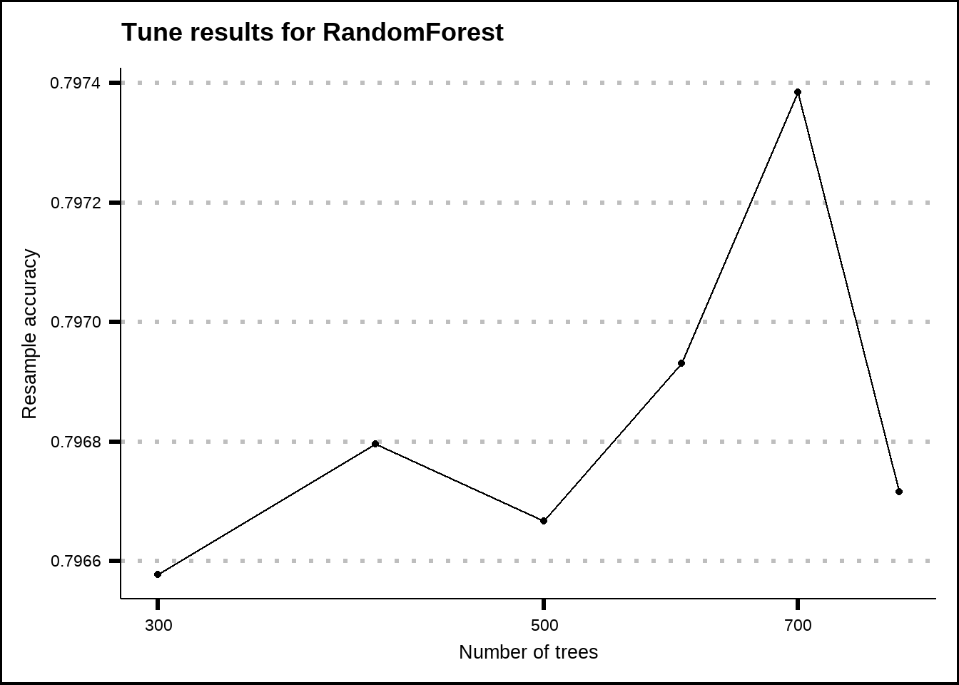 The results from the model tuning indicate that the improvement is very limited with more trees than somewhere around 2000 so I will assume this as the optimal. With tree based models, too much trees can overfit the data so it’s a good idea not to
rf_best_tune <- select_best(rf_final_tune)

rf_final_mod <- rand_forest(trees = 2000, min_n = 5) %>%
  set_mode("classification") %>%
  set_engine("randomForest")

rf_final_wf <- glm_final_wf %>%
  update_model(rf_final_mod)

set.seed(8584)
rf_final_fit <- fit(rf_final_wf, final_train)
rf_fitted <- extract_fit_engine(rf_final_fit)

rf_final_pred <- predict(rf_final_fit, final_test)

confusionMatrix(data = rf_final_pred$.pred_class, reference = final_test$Transported)
#> Confusion Matrix and Statistics
#>
#>           Reference
#> Prediction False True
#>      False   721  186
#>      True    161  671
#>
#>                Accuracy : 0.8005
#>                  95% CI : (0.7809, 0.819)
#>     No Information Rate : 0.5072
#>     P-Value [Acc > NIR] : <2e-16
#>
#>                   Kappa : 0.6007
#>
#>  Mcnemar's Test P-Value : 0.1976
#>
#>             Sensitivity : 0.8175
#>             Specificity : 0.7830
#>          Pos Pred Value : 0.7949
#>          Neg Pred Value : 0.8065
#>              Prevalence : 0.5072
#>          Detection Rate : 0.4146
#>    Detection Prevalence : 0.5216
#>       Balanced Accuracy : 0.8002
#>
#>        'Positive' Class : False
#>
8.9 XGBoost
xgb_final_mod <- boost_tree(trees = 15) %>%
  set_mode("classification") %>%
  set_engine("xgboost")

xgb_final_wf <- glm_final_wf %>%
  update_model(xgb_final_mod)

set.seed(8584)
xgb_final_fit <- fit(xgb_final_wf, final_train)
xgb_fitted <- extract_fit_engine(xgb_final_fit)

xgb_final_pred <- predict(xgb_final_fit, final_test)

confusionMatrix(data = xgb_final_pred$.pred_class, reference = final_test$Transported)
#> Confusion Matrix and Statistics
#>
#>           Reference
#> Prediction False True
#>      False   714  187
#>      True    168  670
#>
#>                Accuracy : 0.7959
#>                  95% CI : (0.7761, 0.8146)
#>     No Information Rate : 0.5072
#>     P-Value [Acc > NIR] : <2e-16
#>
#>                   Kappa : 0.5915
#>
#>  Mcnemar's Test P-Value : 0.3394
#>
#>             Sensitivity : 0.8095
#>             Specificity : 0.7818
#>          Pos Pred Value : 0.7925
#>          Neg Pred Value : 0.7995
#>              Prevalence : 0.5072
#>          Detection Rate : 0.4106
#>    Detection Prevalence : 0.5181
#>       Balanced Accuracy : 0.7957
#>
#>        'Positive' Class : False
#>
8.10 C5
c50_final_mod <- boost_tree(trees = 15) %>%
  set_mode("classification") %>%
  set_engine("C5.0")

c50_final_wf <- glm_final_wf %>%
  update_model(c50_final_mod)

set.seed(8584)
c50_final_fit <- fit(c50_final_wf, final_train)
c50_fitted <- extract_fit_engine(c50_final_fit)

c50_final_pred <- predict(c50_final_fit, final_test)

confusionMatrix(data = c50_final_pred$.pred_class, reference = final_test$Transported)
#> Confusion Matrix and Statistics
#>
#>           Reference
#> Prediction False True
#>      False   708  188
#>      True    174  669
#>
#>                Accuracy : 0.7918
#>                  95% CI : (0.772, 0.8107)
#>     No Information Rate : 0.5072
#>     P-Value [Acc > NIR] : <2e-16
#>
#>                   Kappa : 0.5835
#>
#>  Mcnemar's Test P-Value : 0.4944
#>
#>             Sensitivity : 0.8027
#>             Specificity : 0.7806
#>          Pos Pred Value : 0.7902
#>          Neg Pred Value : 0.7936
#>              Prevalence : 0.5072
#>          Detection Rate : 0.4071
#>    Detection Prevalence : 0.5152
#>       Balanced Accuracy : 0.7917
#>
#>        'Positive' Class : False
#>
Our score on Kaggle was 0.7898 which is very close to our tuned values. This indicates that our process gives us accurate estimations and now we must consider how we can improve it or select a better model.