3 Handle missing data

The best way to handle missing data is first to visualize it to get a sense of what’s going on.

3.1 Simple but useful features

We’re given several useful bits of information about the data on the competition website that we can apply to create some useful features. By features, I mean new variables that are derived from existing ones. For example, Cabin is comprised of information about the cabin number, the deck and the side and PassengerId contains the passenger group id.

I’ve created a function that derives these new variables from existing ones. It also creates features that count the number of unique categories of different variables by passenger group. Since the passenger group variable is the only one with no missing values, it makes sense to start the exploration of the others based on it. Questions that we could ask are: ‘Is any passenger group travelling from different home planets?’

useful_features <- function(x) {
  x2 <- x %>%
    mutate(PassengerGroup = str_split_i(PassengerId, "_", 1),
           LastName = word(Name, -1),
           Deck = str_split_i(Cabin, "/", 1),
           CabinNumber = str_split_i(Cabin, "/", 2),
           Side = str_split_i(Cabin, "/", 3),
           TotalSpent = RoomService + FoodCourt + ShoppingMall + Spa + VRDeck,
           PassengerCount = 1) %>% # I added this to use as a count variable in visualizations
    group_by(PassengerGroup) %>%
    add_count(PassengerGroup, name = "PassengerGroupSize") %>%
    mutate(HomePlanetsPerGroup = n_distinct(HomePlanet, na.rm = TRUE),
           DestinationsPerGroup = n_distinct(Destination, na.rm = TRUE),
           CabinsPerGroup = n_distinct(Cabin, na.rm = TRUE),
           TotalSpentPerGroup = sum(TotalSpent, na.rm = TRUE),
           CryoSleepsPerGroup = n_distinct(CryoSleep, na.rm = TRUE),
           VIPsPerGroup = n_distinct(VIP, na.rm = TRUE),
           LastNamesPerGroup = n_distinct(LastName, na.rm = TRUE)) %>%
    ungroup() %>%
    mutate(across(.cols = c(HomePlanet, CryoSleep, Destination, VIP, Transported, Deck, Side, HomePlanetsPerGroup,
                            PassengerGroupSize, DestinationsPerGroup, CabinsPerGroup, CryoSleepsPerGroup, VIPsPerGroup,
                            LastNamesPerGroup, PassengerId),
                  .fns = as.factor)) %>%
    mutate(across(.cols = c(CabinNumber, Age, RoomService, FoodCourt, ShoppingMall, Spa, VRDeck, PassengerGroup),
                  .fns = as.integer))
  return(x2)
}

train2 <- useful_features(train)

3.2 Closer look at missing values

A closer look at each variable with missing values gives us more insights. For example, every passenger group always starts from the same home planet. Figure 3.1 shows a sample of passenger groups and their home planets. This is one of the patterns of missingness I alluded to earlier and we can use this information to replace missing HomePlanet values for passengers belonging to a group with a known home planet. This will leave us only with passengers who are travelling alone.

train2 %>%
  group_by(PassengerGroup) %>%
  filter(any(is.na(HomePlanet))) %>%
  ungroup() %>%
  slice_sample(n = 50) %>%
  ggplot(., mapping = aes(x = PassengerGroup, y = PassengerCount, fill = HomePlanet)) +
    geom_col()  +
    labs(title = "Example missing HomePlanet", x = "Passenger group", y = "Number of passengers") +
    scale_y_continuous(breaks = seq(0, 9000, 50)) +
    theme(axis.text.x = element_text(angle = 90, hjust = 1))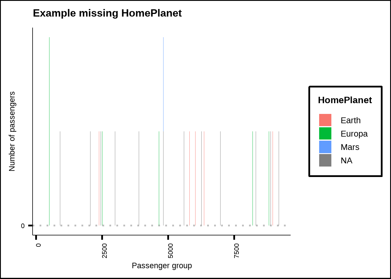

Figure 3.1: Sample of missing values for HomePlanet

We can also see that groups with two or more travelers are never housed in the same cabins as other (non-solo) groups. In other words, a group with two or more passengers can be spread out across several cabins but never share those cabins with other groups of two or more passengers. Figure 3.2 shows a sample. We can use this information to replace missing cabin values.

train2 %>%
  filter(PassengerGroupSize != 1 & Side == "S" & Deck == "G") %>%
  slice_sample(n = 50) %>%
  ggplot(., mapping = aes(x = as.factor(CabinNumber), y = PassengerCount, fill = PassengerGroup)) +
  geom_col() +
  labs(title = "Example missing CabinNumber", x = "Cabin number", y = "Number of passengers") +
  theme(axis.text.x = element_text(angle = 90, hjust = 1), legend.position = "none")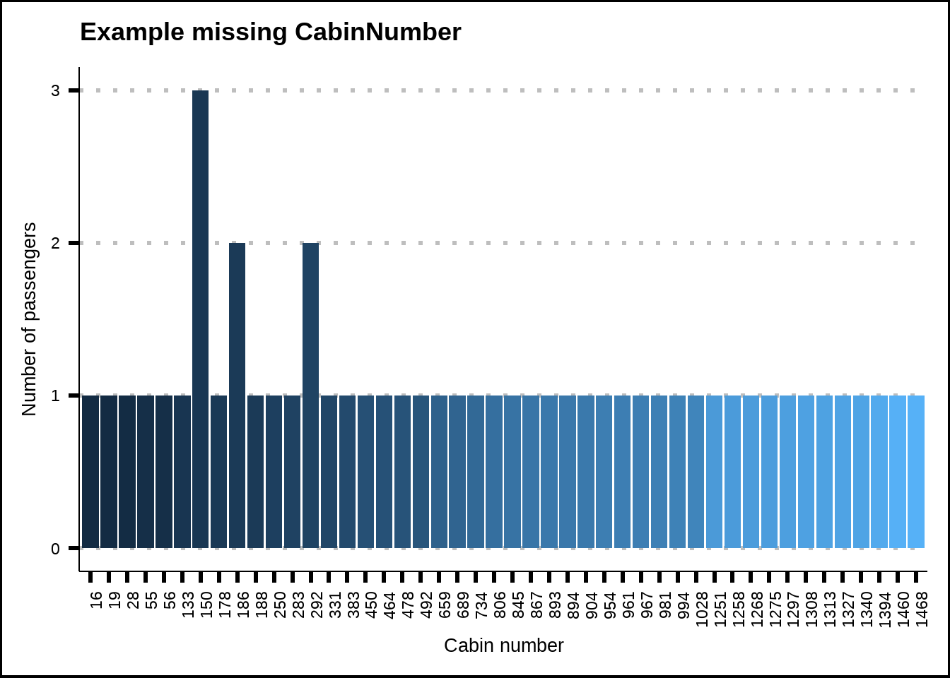

Figure 3.2: Sample of missing values for Cabin

When we look at the new feature Deck, we can see that some decks seem dedicated to passengers from a specific home planet, see Figure 3.4. This helps us replace even more missing values for HomePlanet.

train2 %>%
  ggplot(., mapping = aes(x = CabinNumber, y = as.integer(PassengerGroup), colour = Deck)) +
  geom_point() +
  labs(title = "CabinNumber against PassengerGroup", x = "Cabin number", y = "PassengerGroup") +
  theme(axis.text.x = element_text(angle = 90, hjust = 1))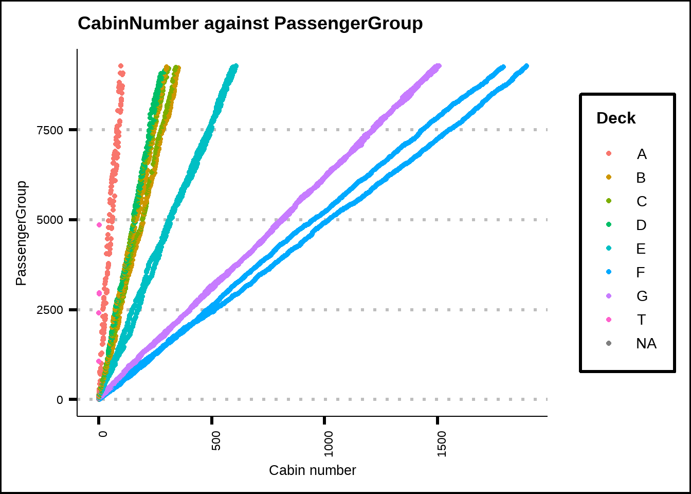

Figure 3.3: Relationsship between Cabin and passenger group.

We see that the relationship between CabinNumber and PassengerGroup is linear so we can use this to replace CabinNumber where Deck is known.

train2 %>%
  group_by(Deck) %>%
  filter(any(is.na(HomePlanet))) %>%
  ungroup() %>%
  ggplot(., mapping = aes(x = Deck, y = PassengerCount, fill = HomePlanet)) +
  geom_col() +
  labs(title = "Missing HomePlanet by Deck", x = "Deck", y = "Number of passengers") +
  scale_y_continuous(breaks = seq(0, 9000, 200)) +
  theme(axis.text.x = element_text(angle = 90, hjust = 1))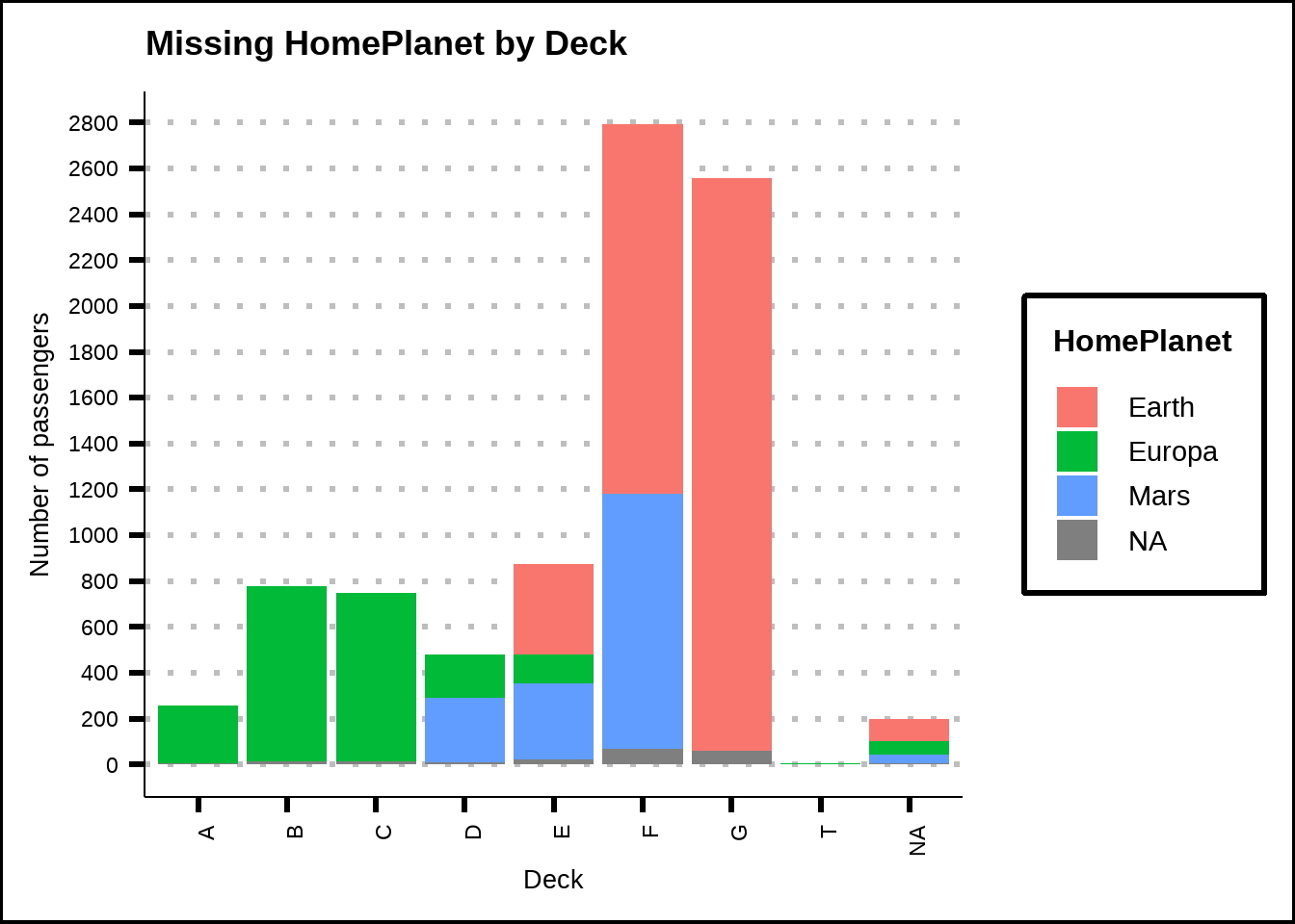

Figure 3.4: Missing values for Deck

We also see that there aren’t any VIPs travelling from Earth so we can use this information to replace missing VIP-values where the home planet is known.

train2 %>%
  ggplot(., mapping = aes(x = HomePlanet, y = PassengerCount, fill = VIP)) +
  geom_col() +
  labs(title = "Missing VIP by HomePlanet", x = "HomePlanet", y = "Number of passengers") +
  scale_y_continuous(breaks = seq(0, 9000, 200)) +
  theme(axis.text.x = element_text(angle = 90, hjust = 1))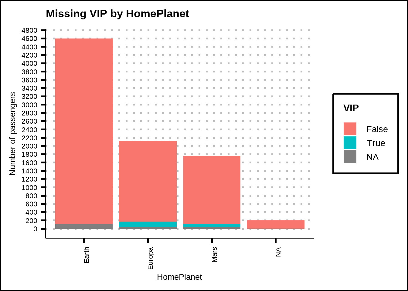

Figure 3.5: Missing values for VIP

We are also told that passengers in cryosleep are confined to their cabins and we must assume that this means they cannot spend any credits on amenities. In other words, we can replace missing amenities with zeroes for passengers in cryo sleep. The reverse is also true: if a passenger has spent credits, the passenger cannot be in cryo sleep.

One last insight we can get from missing data is that passengers of 12 years of age or under don’t spend any credits. We can therefore use this to replace even more missing values for amenities.

train2 %>%
  ggplot(., mapping = aes(x = Age, y = TotalSpent)) +
  geom_col() +
  labs(title = "Missing Age", x = "Age of passengers", y = "TotalSpent") +
  scale_y_continuous(breaks = seq(0, 500000, 50000)) +
  scale_x_continuous(breaks = seq(0, 100, 2)) +
  theme(axis.text.x = element_text(angle = 90, hjust = 1))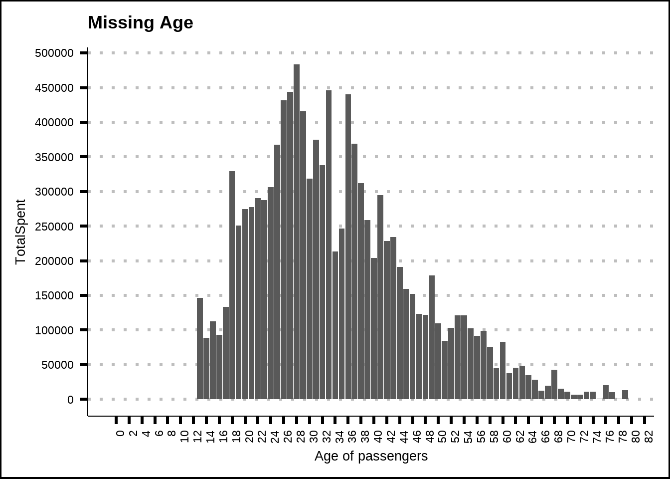

Figure 3.6: Missing values for ameneties

3.3 Replace data with manual rules

I’ve summed up all of these replacement rules in the function below.

my_na_replace <- function(d) {
  cabin_coef <- d %>%
  nest(.by = Deck) %>%
  filter(!is.na(Deck)) %>%
  mutate(cabin_lm = map(.x = data, .f = \(df) lm(CabinNumber ~ PassengerGroup, data = df, na.action = na.exclude)),
         my_tidy = map(.x = cabin_lm, .f = \(m) tidy(m))) %>%
  select(Deck, my_tidy) %>%
  unnest(my_tidy) %>%
  select(Deck, term, estimate) %>%
  pivot_wider(names_from = term, values_from = estimate) %>%
  rename(Intercept = `(Intercept)`, Slope = PassengerGroup)
  
  d2 <- d %>%
    # Replace HomePlanet for passengers in groups where the homeplanet is known from the other passengers
    group_by(PassengerGroup) %>% 
    fill(HomePlanet, .direction = "downup") %>% 
    
    # Replace Cabin by group cabin for groups with group count > 1. Update the Deck, CabinNumber and Side variables.
    mutate(Cabin2 = Cabin) %>%
    fill(data = ., Cabin2, .direction = "downup") %>%
    ungroup() %>%
    mutate(Cabin = if_else(is.na(Cabin) & PassengerGroupSize != 1, Cabin2, Cabin),
           Deck = str_split_i(Cabin, "/", 1),
           CabinNumber = as.integer(str_split_i(Cabin, "/", 2)),
           Side = str_split_i(Cabin, "/", 3)) %>%
    select(-Cabin2) %>%
    
    # Replace remaining CabinNumber with linear relationship with group
    left_join(., cabin_coef, by = "Deck") %>%
    mutate(CabinNumber = if_else(is.na(CabinNumber), Intercept + Slope * PassengerGroup, CabinNumber)) %>%
    select(-Intercept, -Slope) %>%
    
    # Replace HomePlanet if the passenger is housed on a dedicated Deck
    mutate(HomePlanet = if_else(is.na(HomePlanet) & Deck == "G", "Earth", HomePlanet),
           HomePlanet = if_else(is.na(HomePlanet) & Deck %in% c("A", "B", "C"), "Europa", HomePlanet)) %>%
    
    # Replace all of VIPs from Earth to FALSE
    mutate(VIP = if_else(is.na(VIP) & HomePlanet == "Earth", "False", VIP)) %>%
    
    # Replace amenities with zero if CryoSleep is TRUE or if Age <= 12
    # Replace CryoSleep with FALSE if the passenger has spent credits
    mutate(across(.cols = c(RoomService, FoodCourt, ShoppingMall, Spa, VRDeck), 
                  .fns = ~ if_else(condition = CryoSleep == "True" | Age <= 12, true = 0, false = .x, missing = .x)),
           CryoSleep = if_else(TotalSpent > 0 & is.na(CryoSleep), "False", CryoSleep))
  return(d2)
}

train3 <- my_na_replace(train2)
train3 <- useful_features(train3)

plot_na_hclust(train3)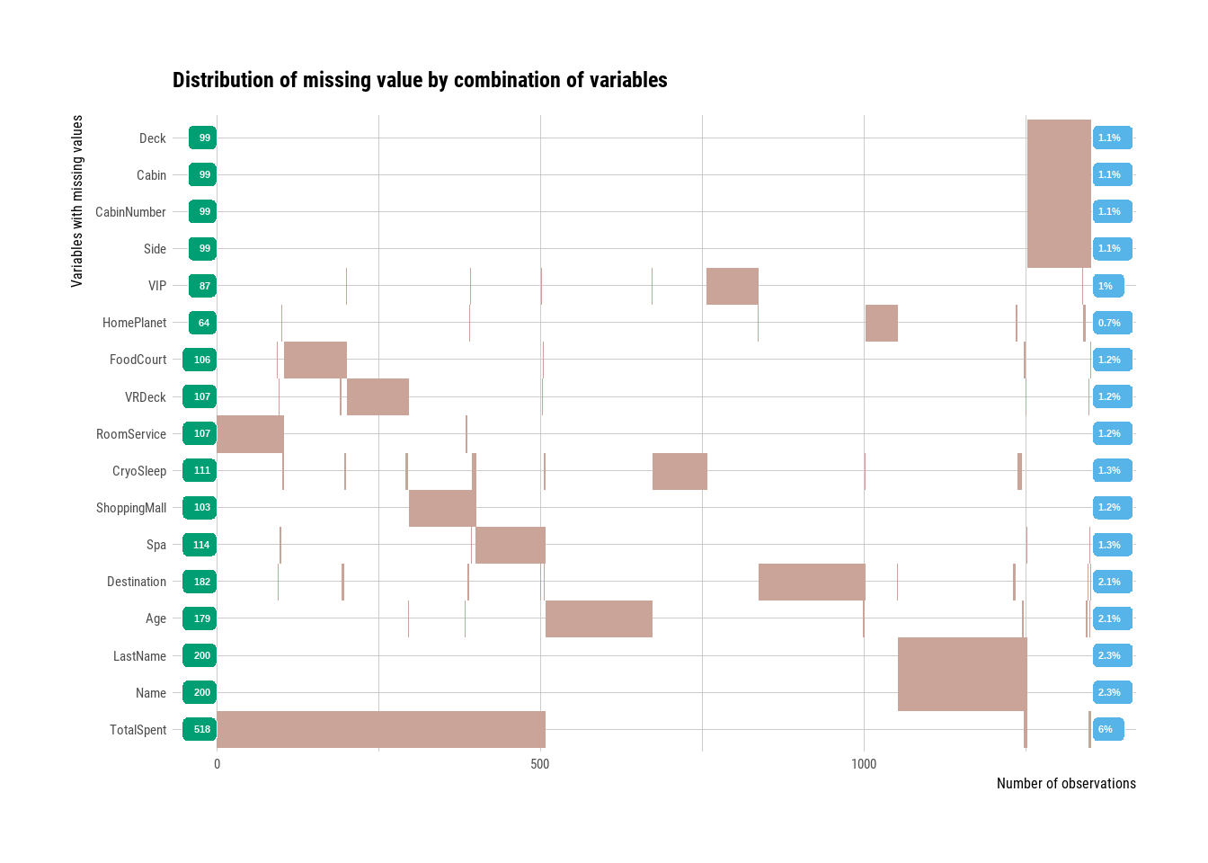

Figure 3.7: Missing values after manual replacement.

We see that we’ve managed to halv the amount of missing values for many variables with our manual replacements. The rest we can handle with imputation.

3.4 Replace data with imputation

Most algorithms require no missing data at all and since we cannot find any more patterns for the missing data, we can use some imputation algorithms to do the rest. I’ve used two: MissRanger and KNN. Since KNN can be sensitive to the scale of the data and outliers, I’ve normalized the numeric data to avoid possible issues with the imputation.

Note that I’ve saved the results for some of these imputations since they can take some time to run. ### MissRanger - Chained Random Forests

rev_normalization <- function(v, rec) { # Custom function that will "unnormalise" numeric values inside mutate(across())
  tidy_rec <- tidy(rec, number = 1)
  v2 <- v * filter(tidy_rec, terms == cur_column() & statistic == "sd")$value + 
    filter(tidy_rec, terms == cur_column() & statistic == "mean")$value
  v3 <- round(v2, 0)
  return(v3)
}

# ranger_norm <- recipe(Transported ~ ., data = train3) %>%
#   step_normalize(all_numeric_predictors()) %>%
#   prep()
# 
# train3_ranger <- ranger_norm %>%
#   bake(new_data = NULL) %>%
#   select(-c(Cabin, Name, LastName, PassengerCount))
# 
# ranger <- missRanger(train3_ranger, formula = . ~ . -PassengerId, seed = 8584, verbose = 0)
# 
# ranger_unnorm <- ranger %>%
#   mutate(across(.cols = c(Age, CabinNumber, RoomService, FoodCourt, ShoppingMall, Spa, VRDeck),
#                 .fns = ~ rev_normalization(.x, ranger_norm)))
# 
# ranger2 <- train3 %>%
#   select(PassengerId, Cabin, Name, LastName, PassengerCount) %>%
#   left_join(ranger_unnorm, ., by = "PassengerId")
# 
# save(ranger2, file = "Extra/MissRanger.RData")
load("Extra/MissRanger.RData")

The missRanger algorithm can impute all of the variables at the same time and there is an option to select an id variable that will be included in the data but not used for imputation. Note that I have excluded the Name variables to improve computation time.

3.4.1 KNN - K-Nearest Neighbors

I use the recipe-package to set up the process of imputation where the step_impute_knn-function allows to specify which variables are to be used for the imputation and which are to be imputed.

train3_for_knn <- train3 %>%
  mutate(across(.cols = where(is.factor), .fns = as.character))

vars_to_impute <- c("HomePlanet", "CryoSleep", "Destination", "Age", "VIP", "RoomService", "FoodCourt", "ShoppingMall",
                    "Spa", "VRDeck", "Deck", "Side", "CabinNumber", "LastName")
vars_for_imputing <- c("HomePlanet", "CryoSleep", "Destination", "Age", "VIP", "RoomService", "FoodCourt",
                              "ShoppingMall", "Spa", "VRDeck", "PassengerGroup", "Deck", "Side", "CabinNumber",
                              "PassengerGroupSize", "DestinationsPerGroup", "CabinsPerGroup",
                              "CryoSleepsPerGroup", "VIPsPerGroup", "LastNamesPerGroup")

train3_noNA <- train3_for_knn[complete.cases(train3_for_knn),]
  
knn_impute_rec <- recipe(Transported ~ ., data = train3_noNA) %>%
  step_normalize(Age, CabinNumber, RoomService, FoodCourt, ShoppingMall, Spa, VRDeck) %>%
  step_impute_knn(recipe = ., all_of(vars_to_impute), impute_with = imp_vars(all_of(vars_for_imputing)), neighbors = 5) 

set.seed(8584)
knn_impute_prep <- knn_impute_rec %>% prep(strings_as_factors = FALSE)

set.seed(8584)
knn_impute_bake <- bake(knn_impute_prep, new_data = train3_for_knn)

knn_impute_res <- knn_impute_bake %>%
  mutate(across(.cols = c(Age, CabinNumber, RoomService, FoodCourt, ShoppingMall, Spa, VRDeck),
                .fns = ~ rev_normalization(.x, knn_impute_prep)))

The KNN-algorithm is very fast and can impute multiple variables at the same time. It can also be relatively easily tuned by changing the number of neighbors the imputation is based on although I’ve used the default = 5.

3.4.2 Comparison of imputation algorithms - numerical variables

Here I use the skimr-package to set up metrics to evaluate and do some data wrangling of the imputated variables to that they can be compared to the non-imputed ones.

my_skim <- skimr::skim_with(numeric = skimr::sfl(min = ~min(., na.rm = TRUE), median = ~median(., na.rm = TRUE), 
                                   mean = ~mean(., na.rm = TRUE), max = ~max(., na.rm = TRUE), 
                                   sd = ~sd(., na.rm = TRUE)), append = FALSE)

no_imp_skim <- train3 %>%
  select(Age, RoomService, FoodCourt, ShoppingMall, Spa, VRDeck, CabinNumber) %>%
  my_skim(.)

ranger_skim <- ranger2 %>%
  select(Age, RoomService, FoodCourt, ShoppingMall, Spa, VRDeck, CabinNumber) %>%
  my_skim(.)

knn_skim <- knn_impute_res %>%
  select(Age, RoomService, FoodCourt, ShoppingMall, Spa, VRDeck, CabinNumber) %>%
  my_skim(.)

sd_skim <- bind_cols("Variable" = no_imp_skim$skim_variable, "No imp" = no_imp_skim$numeric.sd, 
                     "MissRanger" = ranger_skim$numeric.sd,  "KNN" = knn_skim$numeric.sd) %>%
  pivot_longer(., cols = !Variable, names_to = "Metric", values_to = "Standard_deviation")

mean_skim <- bind_cols("Variable" = no_imp_skim$skim_variable, "No imp" = no_imp_skim$numeric.mean, 
                     "missRanger" = ranger_skim$numeric.mean, "KNN" = knn_skim$numeric.mean) %>%
  pivot_longer(., cols = !Variable, names_to = "Metric", values_to = "Mean")

sd_skim %>%
  filter(Metric != "No imp") %>%
  ggplot(., mapping = aes(x = Metric, y = Standard_deviation)) +
  geom_point() +
  geom_hline(data = sd_skim %>% filter(Metric == "No imp"), aes(yintercept = Standard_deviation, colour = "orange")) +
  lims(y = c(0, NA)) +
  facet_wrap(~Variable, scales = "free") +
  scale_colour_discrete(name = "Non-imputed", labels = "sd", type = "orange")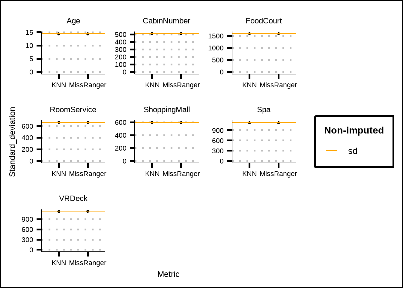

Figure 3.8: Comparisson of standard deviation for numerical values before and after imputation

The standard deviation for our numeric variables isn’t affected by the imputation, although this was expected since we only have 1% of missing data. The same is true for the mean, as can be seen in Figure 3.9.

mean_skim %>%
  filter(Metric != "No imp") %>%
  ggplot(., mapping = aes(x = Metric, y = Mean)) +
  facet_wrap(~Variable, scales = "free") +
  geom_point() +
  geom_hline(data = mean_skim %>% filter(Metric == "No imp"), aes(yintercept = Mean, colour = "green")) +
  lims(y = c(0, NA)) +
  scale_colour_discrete(name = "Non-imputed", labels = "mean", type = "green")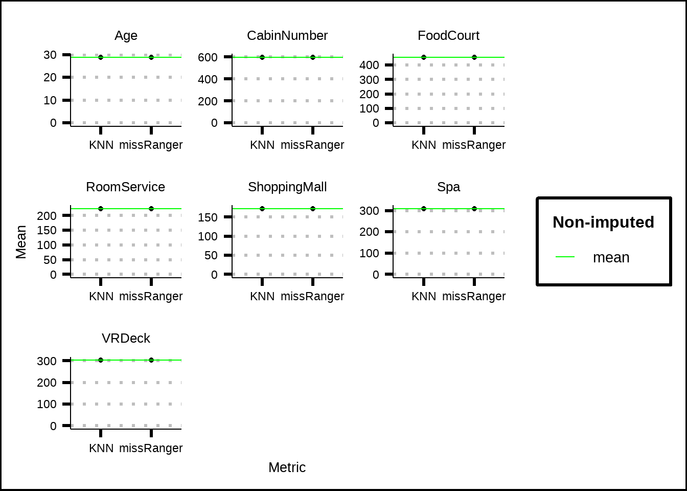

Figure 3.9: Comparisson of mean for numerical values before and after imputation

3.4.3 Comparison of imputation algorithms - categorical variables

A comparison of proportions of the categorical variables also shows that the imputation seems reasonable and hasn’t introduced any strange values like outliers. Below are two sample comparisons for HomePlanet and CryoSleep but I encourage you (if you follow along this code) to explore each categorical variable seperately.

my_prop_plot <- function(df, v, t) {
  g <- ggplot(data = df, mapping = aes(x = !!sym(t), fill = !!sym(v))) +
    geom_bar() +
    geom_text(aes(by = as.factor(!!sym(t))), stat = "prop", position = position_stack(vjust = 0.5)) +
    labs(title = deparse(substitute(df)), x = t, y = "Number of passengers") +
    scale_y_continuous(breaks = seq(0, 9000, 500)) +
    theme(axis.text.x = element_text(angle = 90, hjust = 1))
  return(g)
}

h1 <- my_prop_plot(train3, "HomePlanet", "Transported")
h2 <- my_prop_plot(ranger2, "HomePlanet", "Transported")
h3 <- my_prop_plot(knn_impute_res, "HomePlanet", "Transported")

(h1 | h2 | h3) + plot_layout(guides = "collect", axis_titles = "collect")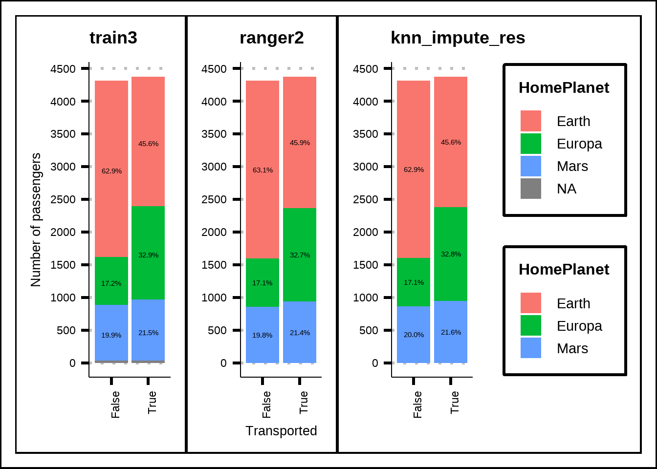

Figure 3.10: Imputed distribution for HomePlanet compared to no imputation

c1 <- my_prop_plot(train3, "CryoSleep", "Transported")
c2 <- my_prop_plot(ranger2, "CryoSleep", "Transported")
c3 <- my_prop_plot(knn_impute_res, "CryoSleep", "Transported")

(c1 | c2 | c3) + plot_layout(guides = "collect", axis_titles = "collect")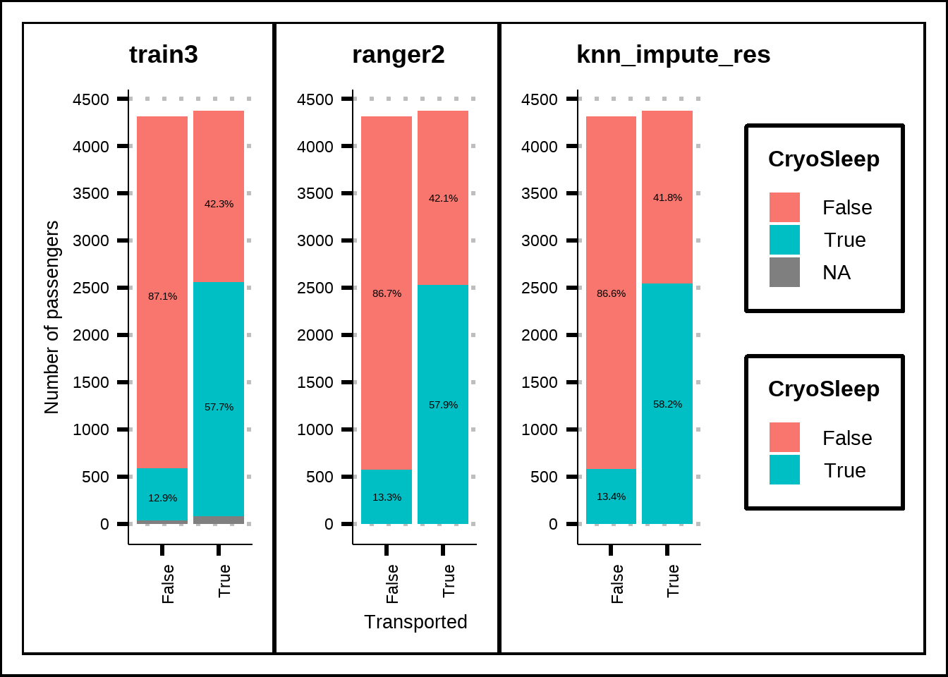

Figure 3.11: Imputed distribution for HomePlanet compared to no imputation

3.4.4 Do the imputated values break any “rules”?

One last thing we must do before we accept the imputed values is to check whether the imputation has managed to adhere to the ‘rules’ we discovered earlier that we used for our manual replacement of NA-values. I use a modified version of the useful_features-function below to update the simple features.

useful_features2 <- function(x) {
  x2 <- x %>%
    mutate(TotalSpent = RoomService + FoodCourt + ShoppingMall + Spa + VRDeck) %>%
    group_by(PassengerGroup) %>%
    add_count(PassengerGroup, name = "PassengerGroupSize") %>%
    mutate(HomePlanetsPerGroup = n_distinct(HomePlanet, na.rm = TRUE),
           DestinationsPerGroup = n_distinct(Destination, na.rm = TRUE),
           CabinsPerGroup = n_distinct(Cabin, na.rm = TRUE),
           TotalSpentPerGroup = sum(TotalSpent, na.rm = TRUE),
           CryoSleepsPerGroup = n_distinct(CryoSleep, na.rm = TRUE),
           VIPsPerGroup = n_distinct(VIP, na.rm = TRUE),
           LastNamesPerGroup = n_distinct(LastName, na.rm = TRUE)) %>%
    ungroup() %>%
    mutate(across(.cols = c(HomePlanet, CryoSleep, Destination, VIP, Transported, Deck, Side, HomePlanetsPerGroup,
                            PassengerGroupSize, DestinationsPerGroup, CabinsPerGroup, CryoSleepsPerGroup, VIPsPerGroup,
                            LastNamesPerGroup, PassengerGroup, PassengerId),
                  .fns = as.factor)) %>%
    mutate(across(.cols = c(CabinNumber, Age, RoomService, FoodCourt, ShoppingMall, Spa, VRDeck),
                  .fns = as.integer))
  return(x2)
}

check_knn <- useful_features2(knn_impute_res)

check_knn %>%
  filter(HomePlanetsPerGroup != 1) %>%
  select(PassengerId, HomePlanet, HomePlanetsPerGroup)
#> # A tibble: 0 × 3
#> # ℹ 3 variables: PassengerId <fct>, HomePlanet <fct>,
#> #   HomePlanetsPerGroup <fct>

The imputation didn’t seem to break the rule where every passenger group travels from the same planet, which is great.

check_knn %>%
  filter(Age <= 12 & TotalSpent > 0) %>%
  select(PassengerId, CryoSleep, Age, RoomService, FoodCourt, ShoppingMall, Spa, VRDeck, TotalSpent)
#> # A tibble: 0 × 9
#> # ℹ 9 variables: PassengerId <fct>, CryoSleep <fct>,
#> #   Age <int>, RoomService <int>, FoodCourt <int>,
#> #   ShoppingMall <int>, Spa <int>, VRDeck <int>,
#> #   TotalSpent <dbl>

check_knn %>%
  filter(CryoSleep == "True" & TotalSpent > 0) %>%
  select(PassengerId, CryoSleep, RoomService, FoodCourt, ShoppingMall, Spa, VRDeck, TotalSpent)
#> # A tibble: 5 × 8
#>   PassengerId CryoSleep RoomService FoodCourt ShoppingMall
#>   <fct>       <fct>           <int>     <int>        <int>
#> 1 0115_01     True                0         0            0
#> 2 2390_01     True                0         0            3
#> 3 5157_01     True              814        12            2
#> 4 7314_01     True                0         0            0
#> 5 7512_01     True                5       598           18
#> # ℹ 3 more variables: Spa <int>, VRDeck <int>,
#> #   TotalSpent <dbl>

The imputation didn’t break the rule where passengers that are <=12 years old don’t spend any credits but it did break the rule where passengers that are in cryo sleep can’t spend credits.

check_knn %>%
  filter(Deck %in% c("A", "B", "C") & HomePlanet != "Europa" | Deck == "G" & HomePlanet != "Earth") %>%
  select(PassengerId, HomePlanet, Deck)
#> # A tibble: 23 × 3
#>    PassengerId HomePlanet Deck 
#>    <fct>       <fct>      <fct>
#>  1 0101_01     Mars       G    
#>  2 0355_01     Earth      B    
#>  3 0525_01     Earth      C    
#>  4 0826_01     Earth      B    
#>  5 0833_01     Europa     G    
#>  6 0932_01     Mars       G    
#>  7 1041_01     Europa     G    
#>  8 1095_01     Europa     G    
#>  9 1134_01     Europa     G    
#> 10 1645_01     Europa     G    
#> # ℹ 13 more rows

check_knn %>%
  filter(VIP == "True" & HomePlanet == "Earth") %>%
  select(PassengerId, HomePlanet, VIP)
#> # A tibble: 0 × 3
#> # ℹ 3 variables: PassengerId <fct>, HomePlanet <fct>,
#> #   VIP <fct>

Another rule that was broken regards the Deck variable where some passengers have been imputed as being housed on decks despite travelling from the ‘wrong’ homeplanet for that deck. We can deal with this in a general function that checks for all the ‘rules’ and adjusts.

fix_knn <- function(df) {
  amenities_summary <- df %>%
    filter(Age > 12 & TotalSpent > 0) %>%
    summarise(mean_age = round(mean(Age), 0), .by = c(CryoSleep, Deck))
  
  wrong_age <- df %>%
    filter(Age <= 12 & TotalSpent > 0) %>%
    left_join(., amenities_summary, by = c("CryoSleep", "Deck")) %>%
    select(PassengerId, mean_age)
  
  wrong_planet <- df %>%
    filter(HomePlanetsPerGroup != 1) %>%
    select(PassengerId, PassengerGroup, HomePlanet) %>%
    group_by(PassengerGroup) %>%
    mutate(HomePlanet_correct = first(HomePlanet)) %>%
    ungroup() %>%
    select(PassengerId, HomePlanet_correct)
  
  wrong_deck <- df %>%
    filter(Deck %in% c("A", "B", "C", "G")) %>%
    mutate(Deck_correct = case_when(Deck %in% c("A", "B", "C") & HomePlanet == "Earth" ~ "G",
                                    Deck %in% c("A", "B", "C") & HomePlanet == "Mars" ~ "F",
                                    Deck == "G" & HomePlanet == "Mars" ~ "F",
                                    Deck == "G" & HomePlanet == "Europa" ~ "C", .default = Deck)) %>%
    select(PassengerId, Deck_correct)
  
  res <- df %>%
  left_join(., wrong_age, by = "PassengerId") %>%
  left_join(., wrong_planet, by = "PassengerId") %>%
  left_join(., wrong_deck, by = "PassengerId") %>%
  mutate(Age = if_else(Age <= 12 & TotalSpent > 0, mean_age, Age),
         RoomService = if_else(CryoSleep == "True", 0, RoomService),
         FoodCourt = if_else(CryoSleep == "True", 0, FoodCourt),
         ShoppingMall = if_else(CryoSleep == "True", 0, ShoppingMall),
         Spa = if_else(CryoSleep == "True", 0, Spa),
         VRDeck = if_else(CryoSleep == "True", 0, VRDeck),
         HomePlanet = if_else(HomePlanetsPerGroup != 1, HomePlanet_correct, HomePlanet),
         Deck_correct = coalesce(Deck_correct, Deck),
         Deck = Deck_correct) %>%
  select(-mean_age, -HomePlanet_correct, -Deck_correct)
  
  return(res)
}

fixed_knn <- fix_knn(check_knn)
train4 <- useful_features2(fixed_knn)

plot_na_hclust(train4)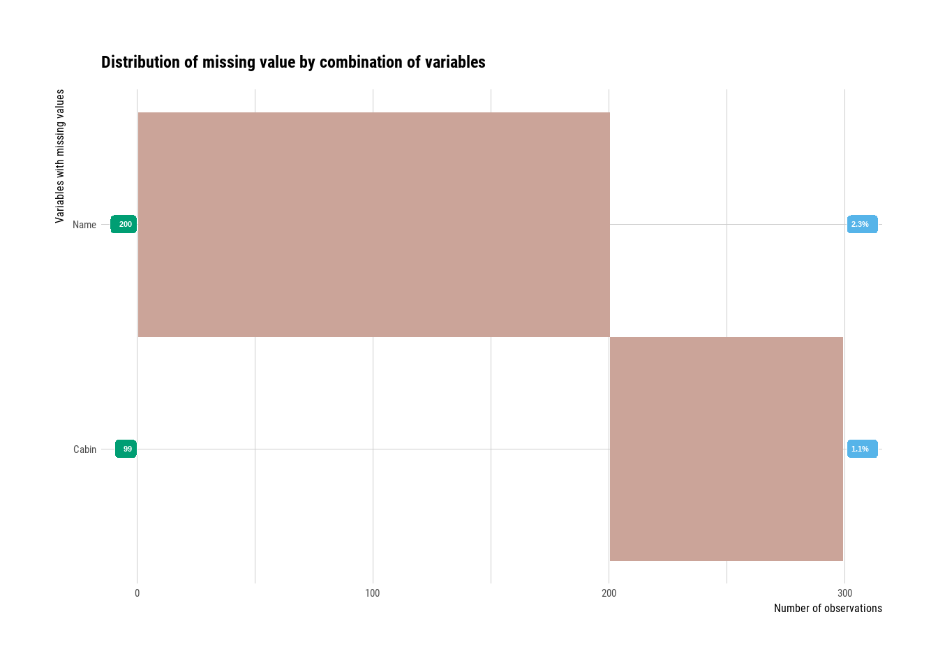

Figure 3.12: Missing values overview after imputation

The only missing values are now in the variables that we won’t use for modelling (we’ll use features derived from them instead).