2 Early data exploration

2.1 Overview of the data

The data has already been divided into train and test sets so let’s load them and get a sense of how the train data looks like. We’ll leave the test data (won’t even look at it) until the end.

Let’s first get a sense of the train data.

train <- read.csv("train.csv", na.strings = "")
str(train)
#> 'data.frame':    8693 obs. of  14 variables:
#>  $ PassengerId : chr  "0001_01" "0002_01" "0003_01" "0003_02" ...
#>  $ HomePlanet  : chr  "Europa" "Earth" "Europa" "Europa" ...
#>  $ CryoSleep   : chr  "False" "False" "False" "False" ...
#>  $ Cabin       : chr  "B/0/P" "F/0/S" "A/0/S" "A/0/S" ...
#>  $ Destination : chr  "TRAPPIST-1e" "TRAPPIST-1e" "TRAPPIST-1e" "TRAPPIST-1e" ...
#>  $ Age         : num  39 24 58 33 16 44 26 28 35 14 ...
#>  $ VIP         : chr  "False" "False" "True" "False" ...
#>  $ RoomService : num  0 109 43 0 303 0 42 0 0 0 ...
#>  $ FoodCourt   : num  0 9 3576 1283 70 ...
#>  $ ShoppingMall: num  0 25 0 371 151 0 3 0 17 0 ...
#>  $ Spa         : num  0 549 6715 3329 565 ...
#>  $ VRDeck      : num  0 44 49 193 2 0 0 NA 0 0 ...
#>  $ Name        : chr  "Maham Ofracculy" "Juanna Vines" "Altark Susent" "Solam Susent" ...
#>  $ Transported : chr  "False" "True" "False" "False" ...

There are 8693 observations and 14 variables where “Transported” is the response. The specifics on the different variables are explained in detail on the competition website so I won’t repeat them here. It’s enough to note that there is a mix of categorical and numerical variables and that our response is a binary classification (True or False).

2.2 Do some variables have zero or near-zero variance?

One of the first things that might be useful to check is whether any of the variables have zero or near-zero variance. A zero variance variable is one where all rows have the same value (imagine a variable where all rows are just the number 1). Such variables are not useful for prediction since they don’t change in any way with the response.

Their close cousin are the near-zero variances where a high percentage of the rows have the same value but a few don’t. This can be particularly problematic when we want to do repeated cross validation where we divide the data into subdata to test our models. Some of these subdata might then have zero variance while others might get a high variance for the same variable.

nearZeroVar(train, saveMetrics = TRUE) %>% rownames_to_column() %>% filter(nzv)
#>   rowname freqRatio percentUnique zeroVar  nzv
#> 1     VIP  41.66332    0.02300702   FALSE TRUE

Only the VIP variable has near-zero variation (2.3% of all rows). We’ll see if this becomes an issue later in our process.

2.3 Frequency distribution of all variables

Let’s see how the values of the different variables are distributed.

sjPlot::plot_frq(train, Transported, type = "histogram")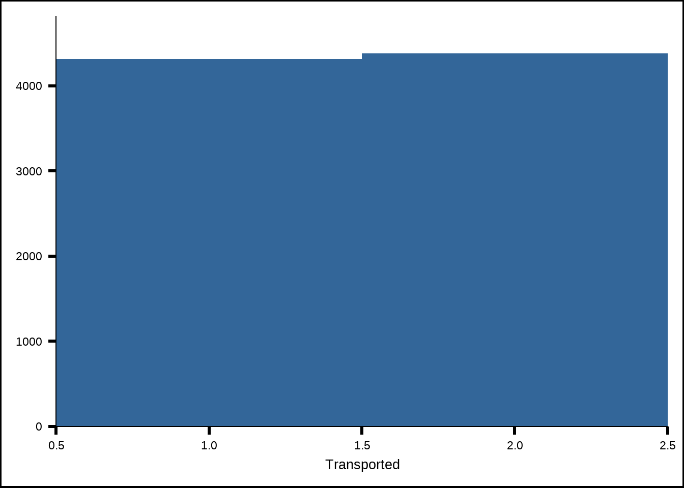

Figure 2.1: Distribution of the response

The response in the training set is balanced which is good and means we don’t need to do any under- or oversampling to balance it. A balanced response is necessary for tuning many models since it makes the metrics we tune against make more sense. If there was a great unbalance in the true responses vs the false ones, then metrics like accuracy might be distorted since even random guesses might give us high accuracy just from the fact that the distirbution is unbalanced.

my_frq <- sjPlot::plot_frq(train, type = "histogram")

save_plot <- function(p, i) {
  ggsave(filename = paste0("Variable", i, ".png"), plot = p, path = "Extra/")
}

# plotsToSVG <- walk2(.x = my_frq, .y = seq_along(my_frq), .f = save_plot)
plotsToSVG <- map(1:length(my_frq), .f = \(i) paste0("Extra/Variable", i, ".png"))
slickR::slickR(plotsToSVG, height = "480px", width = "672px") +
  slickR::settings(slidesToShow = 1, dots = TRUE)

Figure 2.2: Distribution of the predictor variables

All of the numeric variables are right-skewed, which means they have outliers to the right of the horizontal axis and the amenities (RoomService, FoodCourt etc) have a high proportion of zero values. The difference in scales is also large. We will need to apply some kind of preproces to scale them down to help out models like K-nearest-neighbors (KNN). We might also need to add binary features (yes/no or 1/0) for the amenities that are zero to perhaps help the models differentiate them from the rest.

The Cabin and Name variables have a near uniform distribution which implies that they either won’t have much predictive power by themselves or could even reduce the accuracy by introducing unnecessary noise to the model. We will either have to derive features from these variables or not include them in the models.

2.4 Correlation between the variables

train %>%
  na.omit(.) %>%
DataExplorer::plot_correlation(., type = "all", theme_config = list(axis.text.x = element_text(angle = 90)))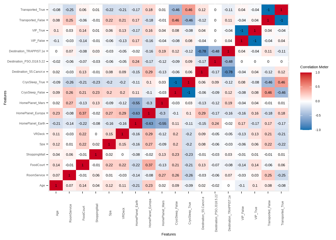

Figure 2.3: Correlation between numerical predictor variables

We see that there’s some relatively high correlation between home planets and destinations as well as a moderate correlation between CryoSleep and Transported which already gives us a hint that CryoSleep might be important. Otherwise, the variables seem relatively uncorrelated which is a good thing since some models cannot handle variables that are too correlated.

2.5 Overview of missing values

plot_na_hclust(train)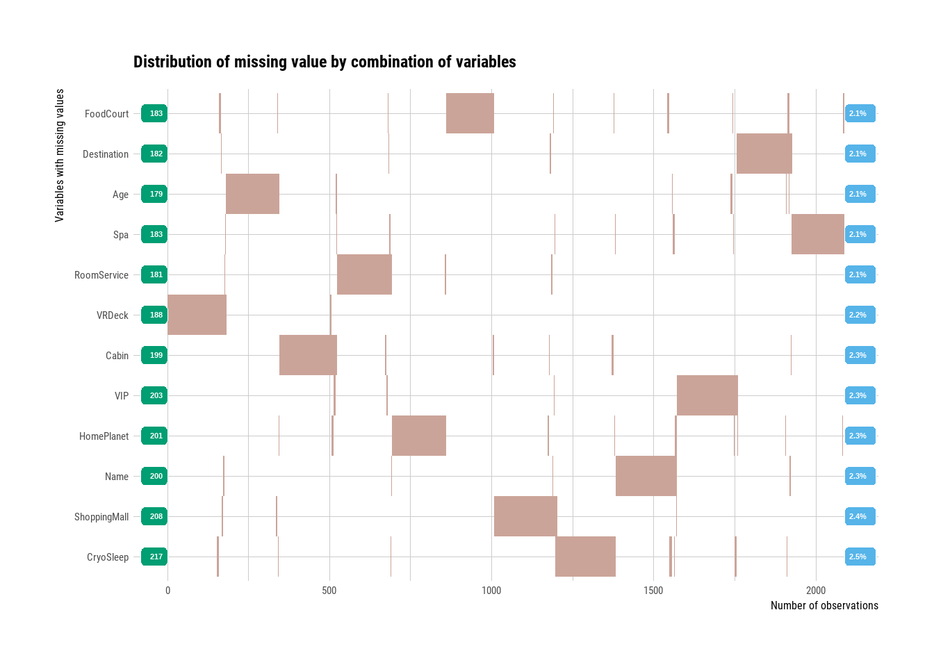

Figure 2.4: Missing values overview

All of the predictor variables have around 2% missing data which is relatively low. When we cluster the missing values, we can also see that most don’t overlap which suggests that they’re missing at random and not due to some specific pattern. This tells us that we can probably find a suitable algorithm to help us impute the missing values based on the non-missing values. Had there been a pattern or clusters of missing data, we’d have to explore further to uncover the reasons for such non-random missingness.

However, we will see in our exploration of the data that there might be some pattern missingness, or at least values that are missing that can be inferred from the others.

1 Introduction

3 Handle missing data