6 Interactions

So far we’ve only created features from single variables but what about the effects of two variables together? Would it help our models if we added an interaction effect between for example HomePlanet and Destination to create the new feature HomeDestination? What about other such interactions?

In the previous competition for the Titanic of 1912, the sex of a passenger mattered (women more likely to survive) and the ticket class mattered (first class more likely to survive) but the interaction “woman in first class” had an almost 100% of survival and this interaction improved the model (if I remember correctly). We want to discover if such interactions exist between the variables that we have for our space odyssey.

Of course, we won’t know the extent of the improvement until we test the interaction effects in various models. Some models inherently discover interactions (like tree-models) and the addition of interaction effects might not matter while it might matter for others.

6.1 Visual exploration of interactions

Since we only have a few categorical variables, let’s visualize all possible interactions. Here I use the default glm logistic regression model where the formula: Transported ~ (.)^2 that amounts to Outcome ~ Variable_1 + Variable_2 + Variable_1 x Variable_2

plot_simple_int <- function(df, v1, v2) {
  tmp_vars <- c("Transported", v1, v2)
  tmp_model <- glm(Transported ~ (.)^2, data = df[, tmp_vars], family = binomial())
  p <- interactions::cat_plot(tmp_model, pred = {{ v1 }}, modx = {{ v2 }}, geom = "line", colors = c25,
                       main.title = paste(v1, "and", v2)) +
    theme(text = element_text(size = 40), plot.title = element_text(size = 40))
  return(p)
}

preds_cat <- c("CryoSleep", "HomePlanet", "Destination", "VIP", "Deck", "Side")
pairs_cat <- combn(preds_cat, 2, simplify = FALSE)
c25 <- c("dodgerblue2", "#E31A1C", "green4", "#6A3D9A", "#FF7F00", "black", "gold1", "skyblue2", "#FB9A99", "palegreen2", "#CAB2D6",
  "#FDBF6F", "gray70", "khaki2", "maroon", "orchid1", "deeppink1", "blue1", "steelblue4", "darkturquoise", "green1", "yellow4",
  "yellow3", "darkorange4", "brown") # Had to add extra colours because I couldn't get `cat_plot` to work with defaults

save_plot <- function(p, i) {
  ggsave(filename = paste0("Extra/PairInt", i, ".png"), plot = p)
}

# cat_pair_int_plots <- pairs_cat %>%
#   map(.x = ., .f = \(vp) plot_simple_int(train6, vp[1], vp[2]))
# 
# cat_plots <- walk2(.x = cat_pair_int_plots, .y = seq_along(cat_pair_int_plots), .f = save_plot)
# cat_slick <- map(1:length(cat_pair_int_plots), .f = \(i) paste0("Extra/PairInt", i, ".png"))
# save(cat_slick, file = "Extra/Plots cat.RData")
load("Extra/Plots cat.RData")

slickR::slickR(cat_slick, height = "480px", width = "672px") +
  slickR::settings(slidesToShow = 1, dots = TRUE)

Figure 6.1: Interaction effects for pairs of categorical variables and against the response.

Parallel lines indicate no significant interaction effects while lines that cross indicate a potential for a significant interactions. I’ll highlight a few interactions below.

plot_simple_int(train6, "CryoSleep", "HomePlanet")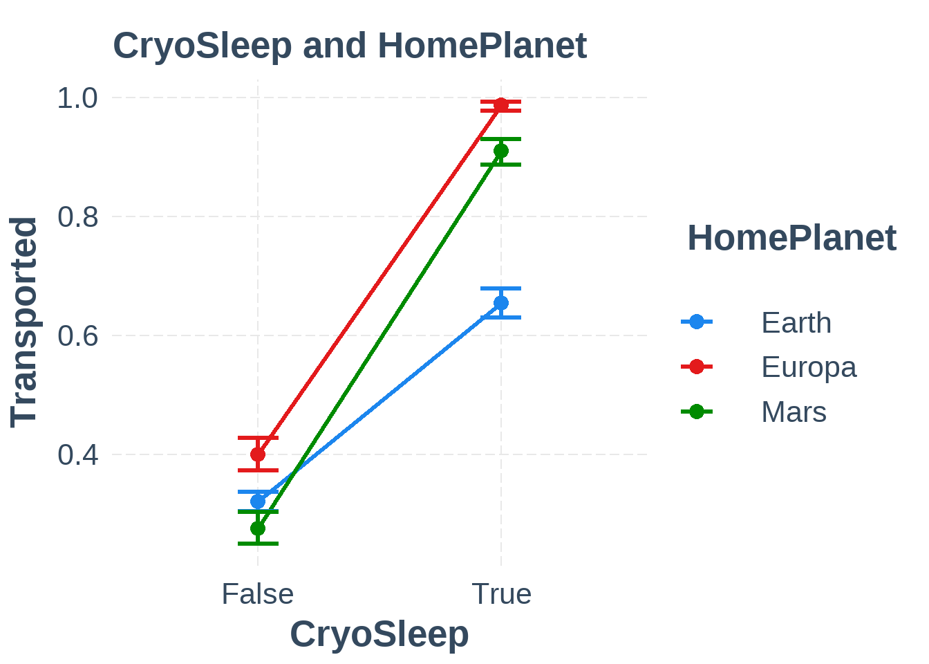

Figure 6.2: Interaction between CryoSleep and HomePlanet

The interaction between CryoSleep and HomePlanet suggests that passengers from Earth are less likely to be transported when in cryosleep which suggests that the interaction CryoSleep & HomePlanet could be useful.

plot_simple_int(train6, "Deck", "Side")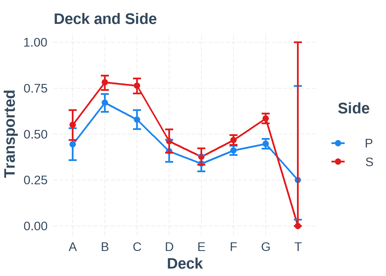

Figure 6.3: Interaction between Deck and Side

The interaction between Deck and Side, however, seems to show only a minor effect, if any.

Figures 6.4 and 6.5 below show all the interaction affects between both numerical and categorical variables.

plot_simple_int2 <- function(df, v1, v2) {
  tmp_vars <- c("Transported", v1, v2)
  tmp_model <- glm(Transported ~ (.)^2, data = df[, tmp_vars], family = binomial())
  p <- interactions::interact_plot(tmp_model, pred = {{ v1 }}, modx = {{ v2 }}, geom = "line", colors = c25,
                       main.title = paste(v1, "and", v2)) +
    scale_x_log10() +
    theme(text = element_text(size = 40), plot.title = element_text(size = 40))
  return(p)
}

preds_num <- c("Age", "RoomService", "FoodCourt", "ShoppingMall", "Spa", "VRDeck", "CabinNumber", "LastNameAsNumber",
               "PassengerGroup", "CryoSleep", "HomePlanet", "Destination", "VIP", "Deck", "Side")
pairs_num <- combn(preds_num, 2, simplify = FALSE)
pairs_num <- pairs_num[1:90]

save_plot2 <- function(p, i) {
  ggsave(filename = paste0("Extra/PairIntNum", i, ".png"), plot = p)
}

# num_pair_int_plots <- pairs_num %>%
#   map(.x = ., .f = \(vp) plot_simple_int2(train6, vp[1], vp[2]))
# 
# int_plots_slick <- walk2(.x = num_pair_int_plots, .y = seq_along(num_pair_int_plots), .f = save_plot2)
# int_plots_slick <- map(1:length(num_pair_int_plots), .f = \(i) paste0("Extra/PairIntNum", i, ".png"))
# save(int_plots_slick, file = "Extra/Plots num.RData")
load("Extra/Plots num.RData")

slickR::slickR(int_plots_slick[1:45], height = "480px", width = "672px") +
  slickR::settings(slidesToShow = 1, dots = TRUE)

Figure 6.4: Interaction effects for pairs of variables against the response. Part 1.

slickR::slickR(int_plots_slick[46:90], height = "480px", width = "672px") +
  slickR::settings(slidesToShow = 1, dots = TRUE)

Figure 6.5: Interaction effects for pairs of variables against the response. Part 2.

Based on what we see in the figures, there seem to be large interaction effects between the numerical variables, especially between some of the amenities. We’ll keep this in mind as we explore further.

6.2 Interaction significance with only variable pairs and their interactions

One problem with the above visual approach is that we don’t know if these interaction effects are real - in the sense they represent some true relationship with the outcome - or if they’re so called false positives - that is, random effects that happened to be present in the training data. For example, does the fact that passengers from Earth seem less likely to be transported even when in cryo sleep reflect some true aspect of the spacetime anomaly that caused the transportation to another dimension or is this pattern just something that happened this time on pure chance? Another way to think of this is: if the Spaceship Titanic were to pass through this spacetime anomaly a thousand times, would the pattern persist?

To explore this further, we must validate some of these effects by cross validation. We will continue to use our simple glm model to model the response against each pair of variables and then compare it to a similar model that includes the interaction term and we’ll use the accuracy metric for comparison.

compare_models_1way <- function(a, b, metric = a$metric[1], ...) { # A customized compare_models function from caret that allows for
  mods <- list(a, b)                                               # a custom t.test adjustment in the diff-function
  rs <- resamples(mods)
  diffs <- diff(rs, metric = metric[1], adjustment = "none", ...)
  res <- diffs$statistics[[1]][[1]]
  return(res)
}

pair_model <- function(df, v1, v2) { # Model without interactions with only two variables
  tmp_vars <- c("Transported", v1, v2)
  set.seed(8584)
  m <- train(Transported ~ ., data = df[, tmp_vars], preProc = NULL, method = "glm", metric = "Accuracy", trControl = ctrl)
  return(m)
}

pair_int_model <- function(df, v1, v2) { # Model with interactions with only two variables
  tmp_vars <- c("Transported", v1, v2)
  set.seed(8584)
  m <- train(Transported ~ (.)^2, data = df[, tmp_vars], preProc = NULL, method = "glm", metric = "Accuracy", trControl = ctrl)
  return(m)
}

preds_cat <- c("CryoSleep", "HomePlanet", "Destination", "Age", "VIP", "Deck", "Side", "RoomService", "FoodCourt", "ShoppingMall",
               "Spa", "VRDeck", "CabinNumber", "LastNameAsNumber", "PassengerGroup")
pairs <- combn(preds_cat, 2, simplify = FALSE)
pairs_cols <- combn(preds_cat, 2, simplify = TRUE) %>%
  t() %>%
  as.data.frame()

ctrl <- trainControl(method = "repeatedcv", repeats = 5, classProbs = TRUE, summaryFunction = multiClassSummary)

# my_cluster <- makeCluster(detectCores() - 1, type = 'SOCK')
# registerDoSNOW(my_cluster)
# 
# no_int_mods <- pairs %>%
#   map(.x = ., .f = \(vp) pair_model(train6, vp[1], vp[2]))
# 
# int_mods <- pairs %>%
#   map(.x = ., .f = \(vp) pair_int_model(train6, vp[1], vp[2]))
# 
# diff_res <- map2(.x = int_mods, .y = no_int_mods, .f = \(m1, m2) compare_models_1way(m1, m2, metric = "Accuracy", 
#                                                                                      alternative = "greater"))
# no_int_acc <- no_int_mods %>%
#   map(.x = ., .f = \(m) getTrainPerf(m)[1, "TrainAccuracy"]) %>%
#   list_c(.)
# 
# int_acc <- int_mods %>%
#   map(.x = ., .f = \(m) getTrainPerf(m)[1, "TrainAccuracy"]) %>%
#   list_c(.)
# 
# save(no_int_acc, file = "Extra/No int acc.RData")
# save(int_acc, file = "Extra/Int acc.RData")
# save(diff_res, file = "Extra/Diff results pairs.RData")
# 
# stopCluster(my_cluster)
# unregister()

load("Extra/No int acc.RData")
load("Extra/Int acc.RData")
load("Extra/Diff results pairs.RData")

diff_res2 <-
  data.frame(Improvement = map_dbl(.x = diff_res, .f = \(est) est$estimate),
             Pvalue = map_dbl(.x = diff_res, .f = \(p) p$p.value)) %>%
  bind_cols(., No_Int_Accuracy = no_int_acc) %>%
  bind_cols(., Int_Accuracy = int_acc) %>%
  bind_cols(., pairs_cols)

diff_res2 %>% 
  filter(Pvalue <= 0.05) %>%
  pivot_longer(cols = c(No_Int_Accuracy, Int_Accuracy)) %>%
  mutate(Pairs = str_c(V1, " and ", V2)) %>%
  ggplot(., aes(x = reorder(Pairs, X = value), y = value, fill = name)) +
  geom_col(position = position_dodge2()) +
  coord_flip() +
  labs(title = "Significant pairwise interactions", x = "Variable pairs", y = "Accuracy") +
  scale_fill_discrete(name = "Models", labels = c("With interactions", "Without interactions")) +
  theme(legend.position = "top")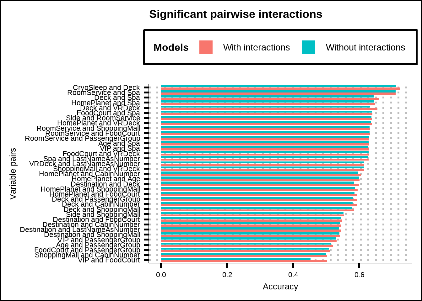

Figure 6.6: Accuracy of GLM-models using only pairs of variables and their interactions.

We see that many variable pairs show significant improvement (based on p-value < 5%), although the improvements are in many cases relatively marginal. Furthermore, we’ve used a cutoff of 5% but without any adjustment which can be problematic since the more tests we run with a 5% cutoff, the higher the chance of finding interactions that have an effect purely by chance (in fact, for our 105 pairs with a 5% cutoff, the chances of getting a false positive is practically guaranteed). We will look at some adjustment methods for p-values to take this into account later.

For now, we can conclude that variables such as CryoSleep & Deck, Deck & Spa, Deck & VRDeck have both high accuracy scores without interactions but seem to be further improved with interactions. Let’s see if these effects persist as we expand the exploration of interactions.

6.3 Interaction significance with entire model and pairwise interactions

One weakness with the above approach is that we’ve looked at variable pairs and their interactions in absence of the other variables so we don’t know how these pairwise interactions contribute to a model with all the other variables. Do the improvements still persist or do some of them become correlated existing variables so that their effects lessen or even introduce noise to the data?

Let’s explore that.

set.seed(8584)
my_split <- initial_split(train6, prop = 0.8)
int_train <- training(my_split) %>%
  mutate(across(.cols = c(PassengerGroup), .fns = as.integer)) %>%
  select(CryoSleep, HomePlanet, Destination, VIP, Deck, Side, Age, RoomService, FoodCourt, ShoppingMall, Spa, VRDeck, CabinNumber,
         LastNameAsNumber, PassengerGroup, Transported)

norm_ctrl <- trainControl(method = "repeatedcv", repeats = 5, classProbs = TRUE, summaryFunction = multiClassSummary)

norm_rec <- recipe(Transported ~ ., data = int_train) %>%
  step_dummy(all_nominal_predictors())

# my_cluster <- makeCluster(detectCores() - 1, type = 'SOCK')
# registerDoSNOW(my_cluster)
# 
# set.seed(8584)
# norm_m <- train(norm_rec, data = int_train, method = "glm", metric = "Accuracy", trControl = norm_ctrl)
# 
# norm_m_acc <- getTrainPerf(norm_m)[1, "TrainAccuracy"]
# 
# int_ctrl <- trainControl(method = "repeatedcv", repeats = 5, classProbs = TRUE, summaryFunction = multiClassSummary)
# 
# int_function <- function(rec, f) {
#   ir <- step_interact(recipe = rec, terms = !!f)
#   return(ir)
# }
# # Map over pairs of vars to create int formulas
# int_form <- map(.x = pairs, .f = \(vp) formula(paste0("~starts_with('", vp[1], "'):starts_with('", vp[2], "')")))
# int_rec <- map(.x = int_form, .f = \(form) int_function(norm_rec, f = form))
# 
# set.seed(8584)
# int_m <- map(.x = int_rec, .f = \(r) train(r, data = int_train, method = "glm", metric = "Accuracy", trControl = int_ctrl))
# 
# int_m_acc <- map_dbl(.x = int_m, .f = \(m) getTrainPerf(m)[1, "TrainAccuracy"])
# 
# anova_res <- map2(.x = int_m, .y =list(norm_m), .f = \(m1, m2) anova(m1$finalModel, m2$finalModel, test = "Chisq"))
# 
# diff_all_res <- map2(.x = int_m, .y = list(norm_m), .f = \(m1, m2) compare_models_1way(m1, m2, metric = "Accuracy",
#                                                                                        alternative = "greater"))
# 
# stopCluster(my_cluster)
# unregister()
# 
# diff_all_res2 <-
#   data.frame(Improvement = map_dbl(.x = diff_all_res, .f = \(est) est$estimate),
#              Resampled_Pvalue = map_dbl(.x = diff_all_res, .f = \(p) p$p.value)) %>%
#   bind_cols(., No_Int_Accuracy = norm_m_acc) %>%
#   bind_cols(., Int_Accuracy = int_m_acc) %>%
#   bind_cols(pairs_cols, .)
# 
# diff_all_res2_anova <- 
#   data.frame(Deviance_improvement = map_dbl(.x = anova_res, .f = \(x) x[["Deviance"]][2]),
#              Traditional_pvalue = map_dbl(.x = anova_res, .f = \(x) x[["Pr(>Chi)"]][2])) %>%
#   bind_cols(., No_Int_Accuracy = norm_m_acc) %>%
#   bind_cols(., Int_Accuracy = int_m_acc) %>%
#   bind_cols(pairs_cols, .)
# 
# save(diff_all_res2_anova, file = "Extra/Anova pairwise interactions with all other variables.RData")
# save(diff_all_res2, file = "Extra/Results pairwise interactions with all other variables.RData")

load("Extra/Anova pairwise interactions with all other variables.RData")
load("Extra/Results pairwise interactions with all other variables.RData")

diff_all_res2_adj <- diff_all_res2 %>%
  mutate(Resampled_pvalue_bh = p.adjust(Resampled_Pvalue, method = "BH"),
         Resampled_pvalue_bon = p.adjust(Resampled_Pvalue, method = "bonferroni"))

If we first look at the results from the ANOVA model comparison, we see that no significant improvements between a model with interactions pairs and one without exist.

diff_all_res2_anova %>%
  filter(Deviance_improvement > 0)
#> [1] V1                   V2                  
#> [3] Deviance_improvement Traditional_pvalue  
#> [5] No_Int_Accuracy      Int_Accuracy        
#> <0 rows> (or 0-length row.names)

Next, if we focus on our resampled performances, we can see that only three interaction effects are statistically significant without any p-value adjustment.

diff_all_res2_adj %>% 
  filter(Resampled_Pvalue <= 0.05) %>%
  pivot_longer(cols = c(Int_Accuracy, No_Int_Accuracy)) %>%
  mutate(Pairs = str_c(V1, " and ", V2)) %>%
  ggplot(., aes(x = reorder(Pairs, X = value), y = value, fill = name)) +
  geom_col(position = position_dodge2()) +
  coord_flip() +
  labs(title = "Unadjusted pairwise interactions", x = "Variable pairs", y = "Accuracy") +
  scale_fill_discrete(name = "Models", labels = c("With interactions", "Without interactions")) +
  theme(legend.position = "top")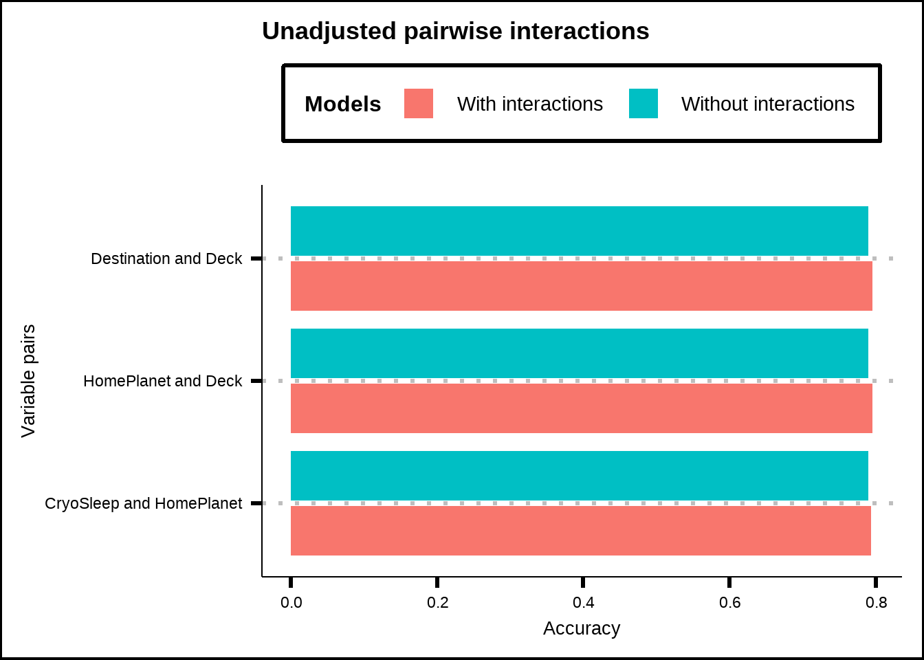

Figure 6.7: Accuracy of GLM-models using pair-interactions together with all other variables for significant interaction effects without any p-value adjustment.

Kuhn and Johnson write that ‘When the interactions that were discovered were included in a broader model that contains other (perhaps correlated) predictors, their importance to the model may be diminished. (…) This might reduce the number of predictors considered important (since the residual degrees of freedom are smaller) but the discovered interactions are likely to be more reliably important to a larger model.’

Let us therefore apply some adjustments.

p_bh <- diff_all_res2_adj %>% 
  filter(Resampled_pvalue_bh <= 0.2) %>%
  pivot_longer(cols = c(Int_Accuracy, No_Int_Accuracy)) %>%
  mutate(Pairs = str_c(V1, " and ", V2)) %>%
  ggplot(., aes(x = reorder(Pairs, X = value), y = value, fill = name)) +
  geom_col(position = position_dodge2()) +
  coord_flip() +
  labs(title = "Benjamini&Hochberg adjusted interactions", x = "Variable pairs", y = "Accuracy") +
  scale_fill_discrete(name = "Models", labels = c("With interactions", "Without interactions"))

p_bon <- diff_all_res2_adj %>% 
  filter(Resampled_pvalue_bon <= 0.2) %>%
  pivot_longer(cols = c(Int_Accuracy, No_Int_Accuracy)) %>%
  mutate(Pairs = str_c(V1, " and ", V2)) %>%
  ggplot(., aes(x = reorder(Pairs, X = value), y = value, fill = name)) +
  geom_col(position = position_dodge2()) +
  coord_flip() +
  labs(title = "Bonferroni adjusted interactions", x = "Variable pairs", y = "Accuracy") +
  scale_fill_discrete(name = "Models", labels = c("With interactions", "Without interactions"))

p_bh / p_bon + plot_layout(guides = "collect", axis_titles = "collect") & theme(legend.position = "top")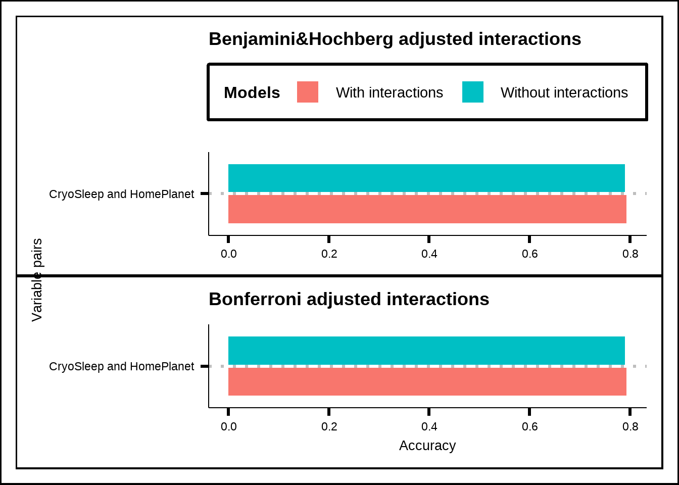

Figure 6.8: Accuracy of GLM-models using pair-interactions together with all other variables for significant interaction effects with Bonferroni and p-value adjustment.

When we adjust our values, only a single interaction effect remains: CryoSleep & HomePlanet. The stricter adjustment is the Bonferroni which multiplies all the p-values with the number of tests (105 in our case) while a less strict adjustment is the Benjamini & Hochberg that sorts the p-values in ascending order and multiplies each one with the total number of tests divided by the p-value’s position (so that the lowest value gets multiplied by 105/1 in our case, the second lowest by 105/2 and so on).

What does this tell us? It suggests that only a few interaction effects seem significant when evaluated together with the entire dataset and that only a single interaction (CryoSleep & HomePlanet) is likely to be truly relevant and not caused by a false positive effect of many tests. We have already seen in Figure 6.2 that the interaction CryoSleep & HomePlanet makes sense and if we look for the other two interactions without p-value adjustment in Figure 6.1 (Deck & HomePlanet as well as Deck & Destination), we see that both of them seem to have large interaction effects.

Let’s add the interaction effects we have so far in a variable that we can use later.

int_vars_very_imp <- diff_all_res2_adj %>% 
  filter(Resampled_Pvalue <= 0.05) %>% 
  select(V1, V2) %>%
  mutate(ForFormula = str_c("starts_with('", V1, "'):starts_with('", V2, "')")) %>%
  mutate(RevFormula = str_c("starts_with('", V2, "'):starts_with('", V1, "')"))

6.4 Penalized regression for interaction exploration

Let’s turn to a different interaction analysis where we’ll use penalized regression to see whether any interactions prove beneficial to the model. Here we use the glmnet-function to first fit a model without interactions and then a model with interactions that we tune with different parameters.

The \(\lambda\) parameter controls the penalty that is applied to different variables to maximize accuracy while the \(\alpha\) controls the weight applied to each penalty function so that \(\alpha = 1\) signifies a Lasso penalty where the penalty is applied to the absolute of the regression coefficient while \(\alpha = 0\) signifies a Ridge penalty where the penalty is applied to the squared coefficient. In our case, the glmnet model allows us to tune for the mix of these factors that gives the best accuracy.

df_pen <- train6 %>%
  select(-c(Cabin, Name, LastName, PassengerCount, HomePlanetsPerGroup)) %>%
    mutate(across(.cols = c(PassengerGroupSize, tidyselect::ends_with("PerGroup")), .fns = as.integer))

set.seed(8584)
my_pen_split <- initial_split(df_pen, prop = 0.8)
pen_train <- training(my_pen_split)
my_pen_folds <- vfold_cv(pen_train, v = 10, repeats = 5)

my_vars <- data.frame(Variables = names(pen_train)) %>%
  mutate(Roles = if_else(Variables == "PassengerId", "id", "predictor"),
         Roles = if_else(Variables == "Transported", "outcome", Roles))

pen_rec <- recipe(x = pen_train, vars = my_vars$Variables, roles = my_vars$Roles) %>%
  step_dummy(all_nominal_predictors()) %>%
  step_zv(all_predictors())

my_acc <- metric_set(accuracy)
pen_ctrl <- control_grid(verbose = TRUE, save_pred = TRUE, save_workflow = TRUE)
pen_grid <- expand.grid(mixture = c(0.2, 0.6, 1), penalty = seq(1e-05, 1e-03, 5e-05))

glmnet_mod <- logistic_reg(penalty = tune(), mixture = tune()) %>%
  set_engine("glmnet")

# my_cluster <- makeCluster(detectCores() - 1, type = 'SOCK')
# registerDoSNOW(my_cluster)
# 
# system.time({
#   set.seed(8584)
#   pen_tune <- glmnet_mod %>%
#     tune_grid(pen_rec, resamples = my_pen_folds, metrics = my_acc, control = pen_ctrl, grid = pen_grid)
# })
# 
# save(pen_tune, file = "Extra/Penalized regression without interactions.RData")
# 
# stopCluster(my_cluster)
# unregister()

load("Extra/Penalized regression without interactions.RData")

pen_best <- fit_best(pen_tune)
pen_coef <- pen_best %>%
  tidy() %>%
  filter(estimate != 0) %>%
  filter(term != "(Intercept)") %>%
  pull(term)

show_best(pen_tune, metric = "accuracy", n = 20) %>%
  mutate(mixture = as.factor(round(mixture, 2))) %>%
  ggplot(aes(x = penalty, y = mean, label = mixture, colour = mixture)) +
  geom_line() +
  geom_point() +
  labs(title = "Tune results without interactions", x = "Lambda penalty", y = "Resample accuracy", colour = "Alpha")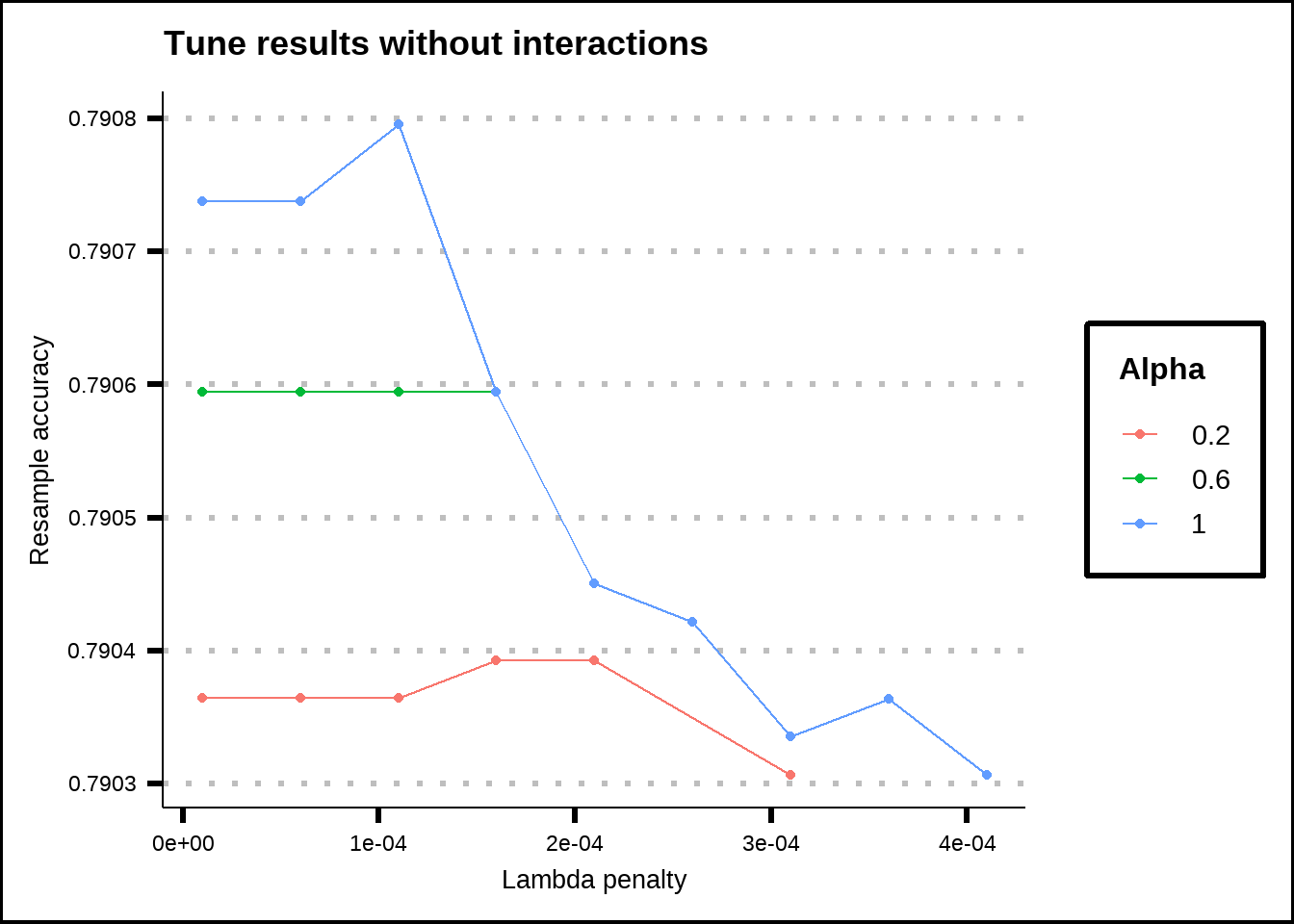

Figure 6.9: Tuning results for a Lasso/Ridge regression without interaction effects.

Without any interaction effects, the regression model favoured the pure Lasso regression (\(\alpha = 1\)) with the penalty \(\lambda = 0.0001\). The most important variables (with the highest coefficients) were in this case HomePlanet, CryoSleep, Deck. The final model used 33 out of 36 variables and the resampled accuracy without any interactions was slightly above 0.79.

If we repeat this process but include interaction effects between the variables that were chosen in the previous section:

int_vars <- pen_coef %>%
  str_split_i(., "_", 1) %>%
  unique() %>%
  combn(., 2, simplify = FALSE)

# Map over pairs of vars to create int formula
int_formula <- map_chr(.x = int_vars, .f = \(vp) paste0("starts_with('", vp[1], "'):starts_with('", vp[2], "')")) %>%
  str_flatten(., collapse = "+") %>%
  paste("~", .) %>%
  as.formula(.)

pen_int_rec <- recipe(x = pen_train, vars = my_vars$Variables, roles = my_vars$Roles) %>%
  step_dummy(all_nominal_predictors()) %>%
  step_interact(int_formula) %>%
  step_zv(all_predictors())

pen_grid <- expand.grid(mixture = c(0.2, 0.6, 1), penalty = seq(1e-04, 1e-02, 5e-04))
  
# my_cluster <- makeCluster(detectCores() - 1, type = 'SOCK')
# registerDoSNOW(my_cluster)
# clusterExport(cl = my_cluster, "int_formula")
# 
# system.time({
#   set.seed(8584)
#   pen_int_tune <- glmnet_mod %>%
#     tune_grid(pen_int_rec, resamples = my_pen_folds, metrics = my_acc, control = pen_ctrl, grid = pen_grid)
# })
# 
# save(pen_int_tune, file = "Extra/Penalized regression with interactions.RData")
# 
# stopCluster(my_cluster)
# unregister()

load("Extra/Penalized regression with interactions.RData")

We see the results from the penalized regression model with interactions below.

show_best(pen_int_tune, metric = "accuracy", n = 40) %>%
  mutate(mixture = as.factor(round(mixture, 2))) %>%
  ggplot(aes(x = penalty, y = mean, label = mixture, colour = mixture)) +
  geom_line() +
  geom_point() +
  labs(title = "Tune results with interactions", x = "Lambda penalty", y = "Resample accuracy", colour = "Alpha")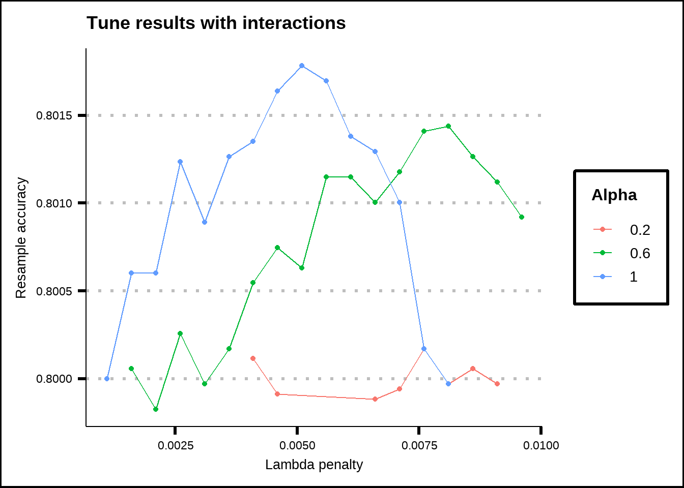

Figure 6.10: Tuning results for a Lasso/Ridge regression with interaction effects.

The regression model still favours the Lasso (\(\alpha = 1\)) but with a higher penalty \(\lambda = 0.005\). Out of 516 total variables including interaction effects, it selected 91 for the best accuracy which was somewhat above 0.80. Compared to the model without interactions effects (accuracy = 0.79), it’s a small improvement.

We can see the top twenty variables from the penalized regression below.

# pen_int_best <- fit_best(pen_int_tune)
# save(pen_int_best, file = "Extra/Best penalized regression with interactions.RData")
load("Extra/Best penalized regression with interactions.RData")
pen_int_coef <- pen_int_best %>%
  tidy()

pen_int_coef %>%
  select(-penalty) %>%
  filter(estimate != 0 & term != "(Intercept)") %>%
  arrange(desc(abs(estimate))) %>%
  slice(1:20) %>%
  ggplot(., aes(x = abs(estimate), y = reorder(term, abs(estimate)))) +
  geom_col() +
  geom_vline(aes(xintercept = 0.50), colour = "red", linetype = "dashed") +
  geom_vline(aes(xintercept = 0.25), colour = "blue", linetype = "dashed") +
  labs(x = "Regression coefficient (abs)", y = "Variable") +
  theme(legend.position = "none")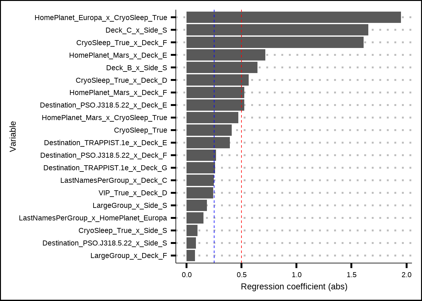

Figure 6.11: Top variables from the Lasso/Ridge regression with interaction effects. The red and blue lines indicate possible (arbitrary) cut-off points for importance.

It’s surprising to see that the strongest effect was between Deck & Side, which we visually inspected in Figure 6.3 where it looked as if the effect of the interaction wasn’t very large. The visual interaction might look deceiving or the effect could be due to overfitting.

The other variables among the 20 most important were almost all interaction effects except CryoSleep and we see returning contenders like CryoSleep & HomePlanet at the top as well as CryoSleep & Deck, Destination & Deck and so on. Although the reduction is gradual, there is a big drop in importance after the first three.

However, since the goal of the competition is to maximise accuracy, there is an argument to be made that all interaction effects could be used to see if they improve model performance.

pen_int_vars <- pen_int_coef %>%
  select(-penalty) %>%
  filter(abs(estimate) != 0 & term != "(Intercept)") %>%
  filter(str_detect(term, "_x_")) %>%
  mutate(V1 = str_split_i(term, "_x_", 1),
         V1 = str_split_i(term, "_", 1),
         V2 = str_split_i(term, "_x_", 2),
         V2 = str_split_i(V2, "_", 1),
         ForFormula = str_c("starts_with('", V1, "'):starts_with('", V2, "')"),
         RevFormula = str_c("starts_with('", V2, "'):starts_with('", V1, "')")) %>%
  select(V1, V2, ForFormula, RevFormula)

save(pen_int_vars, file = "Extra/Best interactions.RData")

6.5 Tree model interactions

A third we can use to indirectly discover interaction effects is by the use of a tree-based model like randomForest. Kuhn and Johnson explain it better in their book but in essence, tree models are by their nature interaction models since they look at thresholds for different variables to split the tree into branches and the splits often involve another variable at the next (or previous) junction.

The results from a randomForest model doesn’t provide interactions themselves but ranks the original variables based on their importance and this can be used to model interaction effects in a second stage.

df_tree <- train6 %>%
  mutate(across(.cols = c(PassengerGroupSize, Solo, LargeGroup, TravelTogether, tidyselect::ends_with("PerGroup")),
                .fns = as.integer))

set.seed(8584)
my_tree_split <- initial_split(df_tree, prop = 0.8)
tree_train <- training(my_tree_split)

my_vars <- data.frame(Variables = names(tree_train)) %>%
  mutate(Roles = if_else(Variables %in% c("PassengerId", "Cabin", "Name", "LastName", "PassengerCount", "HomePlanetsPerGroup"),
                         "id", "predictor"),
         Roles = if_else(Variables == "Transported", "outcome", Roles))

tree_rec <- recipe(x = tree_train, vars = my_vars$Variables, roles = my_vars$Roles) %>%
  step_dummy(all_nominal_predictors()) %>%
  step_zv(all_predictors())

tree_baked <- tree_rec %>%
  prep() %>%
  bake(new_data = NULL) %>%
  select(-c(Cabin, Name, LastName, PassengerCount, HomePlanetsPerGroup))

# my_cluster <- makeCluster(detectCores() - 1, type = 'SOCK')
# registerDoSNOW(my_cluster)
# 
# system.time({
#   rf_mod <- ranger::ranger(Transported ~ . -PassengerId, data = tree_baked, num.trees = 1000, importance = "impurity",
#                    num.threads = detectCores() - 1, seed = 8584)
# })
# 
# save(rf_mod, file = "Extra/Ranger tree model variable importance.RData")
# 
# stopCluster(my_cluster)
# unregister()

load("Extra/Ranger tree model variable importance.RData")

rf_imp <- tibble(Predictor = names(rf_mod$variable.importance),
                 Importance = unname(rf_mod$variable.importance))

ggplot(rf_imp, aes(x = reorder(Predictor, Importance), y = Importance)) +
  geom_bar(stat = "identity") +
  coord_flip() +
  xlab("")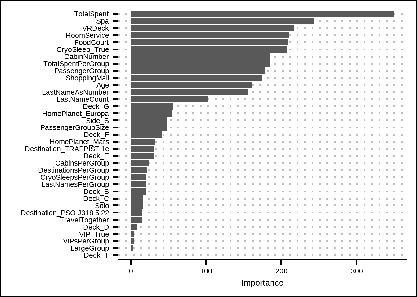

Figure 6.12: Variable importance based on a the ranger tree model

The tree model heavily favours the amenity variables, especially the TotalSpent feature that we’ve created. However, this feature was penalized to zero in our penalized regression, most likely because it correlates to the other amenity variables. All other amenities are, however, represented among the variables from our best penalized results so we’ll stick with them going forward.