8 Final model tuning
The exploration of the data has so far yielded a set of features, including second level interactions, that we think offers the best accuracy. We’ve tested them through several feature selection processes and have gotten some insight on this models performance through resampling evaluations.
Now we must decide which models, or assembly of models, we want to use for our final prediction. There are many different model engines that can handle classification problems, with different pros and cons. Here is a list of the ones we will be using:
| Model | Description |
|---|---|
| Logistic Regression | This is the glm-model that we’ve already used. The logistic regression model is a form of linear model that uses the logit-function to transform a linear equation like \(y = \beta_0 + \beta_1x_1 + \beta_2x_2\) into a logistic equation that would ensure that the probability of the outcome would stay between 0 and 1. The logit function is then used to transform the coefficients fitted to a linear model into a response that can be assigned to discrete values. To assign correct probabilities to different classes, the model uses maximal likelihood estimation. |
| Penalized logistic regression (Lasso/Ridge) | These models are based on linear regression (or logistic, in our case) but have a penalty term that is applied to the regression coefficients in order to maximize the desired metric. When the penalty is the square of the coefficients, it’s called a Rigde regression and when it’s the absolute value, it’s called the Lasso regression (least absolute shrinkage and selection operator). We have used this model in Chapter 6 to find a set of best interaction effects. |
| Generalized Additive Models (GAM) | General additive models or GAM are used to model non-linear relationships using splines which is a way to smoothly interpolate between fixed points using a set of polynomial functions. Instead of a single function that must fit to the entire range of values of a predictor against an outcome, the gam-model uses several polynomials between each spline that are connected and that better describe the relationship. It also makes best estimates for where the splines should be positioned. We have used this type of model in Chapter 5 to show the relationships between numerical variables and the outcome. |
| Support Vector Machines (SVM) | Support vector machines use mapping functions to find hyperplanes that can divide the observations into groups that most accurately fit the outcome class. To find the hyperplane that best classifies the data, the SVM-model can use different functions that are called kernels. There is a linear, polynomial and a radial kernel that we can use to see which one works best on our data. |
| Naive Bayes |
The Exact Bayes model would, for each row of the data, find all other rows that have the exact same set of predictor values and then predict the outcome for that row based on the most probable outcome out of that group. For most datasets, this is impractical since, with enough variables, there wouldn’t be any observations (rows) of data that were exactly the same. The Naive Bayes model assumes instead that the probabilities of each predictor can be calculated independent of the other predictors and then multiplied to get the overall probability of a certain outcome. For example, using CryoSleep and VIP from our dataset, the Naive Bayes model would calculate the probability of CryoSleep = TRUE given Transported = TRUE, which would simply be the proportion of all transported passengers that were also in cryosleep against the number of transported passengers. It would then do the same for VIP = TRUE and multiply these two probabilities with each other was well as the proportion of Transported = TRUE against the total amount of passengers. The resulting probability would then be compared to the its reverse proportions, that is, CryoSleep = TRUE and VIP = TRUE given that Transported = FALSE. The result would be that the higher probability determines how the outcome for that observation (CryoSleep = TRUE and VIP = TRUE) is predict |
| K-nearest neighbors | It has some similarity to the Naive Bayes model in the sense that the algorithm looks for k observations that have similar values and uses the outcome that the neighbors have to predict the new observation. |
| C5.0 | A tree-based model that uses entropy to find the best splits in the data |
| RandomForest |
In a traditional tree-model, the variables are split into branches over many splits until a split point is find that minimizes some criterion, often the Gini impurity that measures the proportions of misclassified records. In the case of two classes, like in our problem, the Gini impurity is given by \(p(1-p)\) where p is the proportion of missclassified records in a partition. Random forest is an extention of this but it uses random sampling of variable sets as well as records to build a forest of decision trees using bootstrap sampling and then aggregates the results across the entire forest of trees. |
| Boosted tree-model (XGBoost) | Boosting is a process of fitting a series of models into an ensamble but adding greater weights to observations whose models performed worse so that each new iteration forces the newer model to train more heavily on the obeservations that had a poorer performance. |
8.1 Complete preprocess
Let’s summarise the entire preprocess for the training data before we get to our models.
8.2 Logistic regression - GLM
glm_final_mod <- logistic_reg() %>%
  set_engine("glm", family = "binomial")

glm_final_wf <- workflow() %>%
  add_recipe(final_rec) %>%
  add_model(glm_final_mod)

glm_control <- control_resamples(save_pred = TRUE, save_workflow = TRUE)

# my_cluster <- snow::makeCluster(detectCores() - 1, type = 'SOCK')
# registerDoSNOW(my_cluster)
# snow::clusterExport(cl = my_cluster, "int_formula")
#
# system.time({
#   set.seed(8584)
#   glm_final_fit_resamples <- fit_resamples(glm_final_wf, final_folds, control = glm_control)
# })
#
# save(glm_final_fit_resamples, file = "Extra/Final GLM tune.RData")
#
# snow::stopCluster(my_cluster)
# unregister()

load("Extra/Final GLM tune.RData")

bind_preds <- function(df, t) {
  res <- map(.x = t, .f = \(x) df %>% mutate("Pred_{{x}}" := if_else(.pred_True < x, "False", "True"), .keep = "none"))
  res <- bind_cols(df, res, .name_repair = "unique_quiet")
  return(res)
}

calc_acc <- function(df) {
  res <- df %>% mutate(across(.cols = starts_with("Pred"), .fns = as.factor),
                       across(.cols = starts_with("Pred"), .fns = ~accuracy_vec(truth = df$Transported, estimate = .x)))
  return(res)
}

glm_resample_pred <- collect_predictions(glm_final_fit_resamples, summarize = TRUE)

glm_thresholds <- seq(0.1, 0.9, 0.05)

glm_resample_acc <- glm_resample_pred %>%
  select(Transported, .pred_False, .pred_True) %>%
  bind_preds(., glm_thresholds) %>%
  calc_acc(.) %>%
  summarise(across(.cols = starts_with("Pred"), .fns = mean)) %>%
  pivot_longer(everything()) %>%
  mutate(name = as.numeric(str_split_i(name, "_", 2)))

glm_p1 <- ggplot(glm_resample_acc, aes(x = name, y = value)) +
  geom_point() +
  labs(x = "Probability threshold", y = "Accuracy") +
  theme(legend.position = "none", axis.text.x = element_text(angle = 90)) +
  scale_x_continuous(breaks = glm_thresholds)

glm_thresholds2 <- seq(0.4, 0.5, 0.01)

glm_resample_acc2 <- glm_resample_pred %>%
  select(Transported, .pred_False, .pred_True) %>%
  bind_preds(., glm_thresholds2) %>%
  calc_acc(.) %>%
  summarise(across(.cols = starts_with("Pred"), .fns = mean)) %>%
  pivot_longer(everything()) %>%
  mutate(name = as.numeric(str_split_i(name, "_", 2)))

glm_p2 <- ggplot(glm_resample_acc2, aes(x = name, y = value)) +
  geom_point() +
  labs(x = "Probability threshold", y = "Accuracy") +
  theme(legend.position = "none", axis.text.x = element_text(angle = 90)) +
  scale_x_continuous(breaks = glm_thresholds2)

glm_p1 + glm_p2 + plot_layout(axis_titles = "collect_y")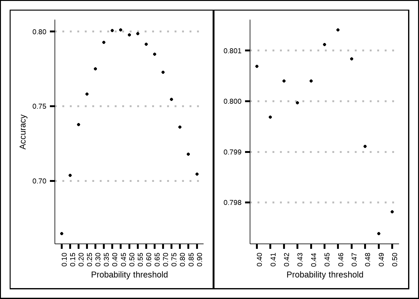
Figure 8.1: Tuning results for the GLM model.
glm_final_fit <- fit(glm_final_wf, final_train)
glm_final_pred <- predict(glm_final_fit, final_test, type = "prob") %>%
  mutate(Prediction = as.factor(if_else(.pred_True < 0.46, "False", "True")))
glm_final_acc <- accuracy_vec(final_test$Transported, glm_final_pred$Prediction)
Based on resamples, it seems that the best threshold for the probability cutoff is 0.46 instead of the normal 0.5. The best accuracy we seem able to get is just above 0.8 with the glm-model.
8.3 Penalized logistic regression - GLMNET
glmnet_final_mod <- logistic_reg(penalty = tune(), mixture = tune()) %>%
  set_engine("glmnet", family = "binomial")

glmnet_final_wf <- glm_final_wf %>%
  update_model(glmnet_final_mod)

my_acc <- metric_set(accuracy)
glmnet_ctrl <- control_grid(save_pred = TRUE, save_workflow = TRUE)
glmnet_grid <- expand.grid(mixture = 1, penalty = seq(1e-07, 1e-04, 1e-06))

# my_cluster <- snow::makeCluster(detectCores() - 1, type = 'SOCK')
# registerDoSNOW(my_cluster)
#
# system.time({
#   set.seed(8584)
#   glmnet_final_tune <- glmnet_final_wf %>%
#     tune_grid(object = ., resamples = final_folds, metrics = my_acc, control = glmnet_ctrl, grid = glmnet_grid)
# })
#
# save(glmnet_final_tune, file = "Extra/Final glmnet tune.RData")
#
# snow::stopCluster(my_cluster)
# unregister()

load("Extra/Final glmnet tune.RData")

show_best(glmnet_final_tune, metric = "accuracy", n = 20) %>%
  mutate(mixture = as.factor(round(mixture, 2))) %>%
  ggplot(aes(x = penalty, y = mean, label = mixture, colour = mixture)) +
  geom_line() +
  geom_point() +
  labs(title = "Final tune results", x = "Lambda penalty", y = "Resample accuracy", colour = "Alpha")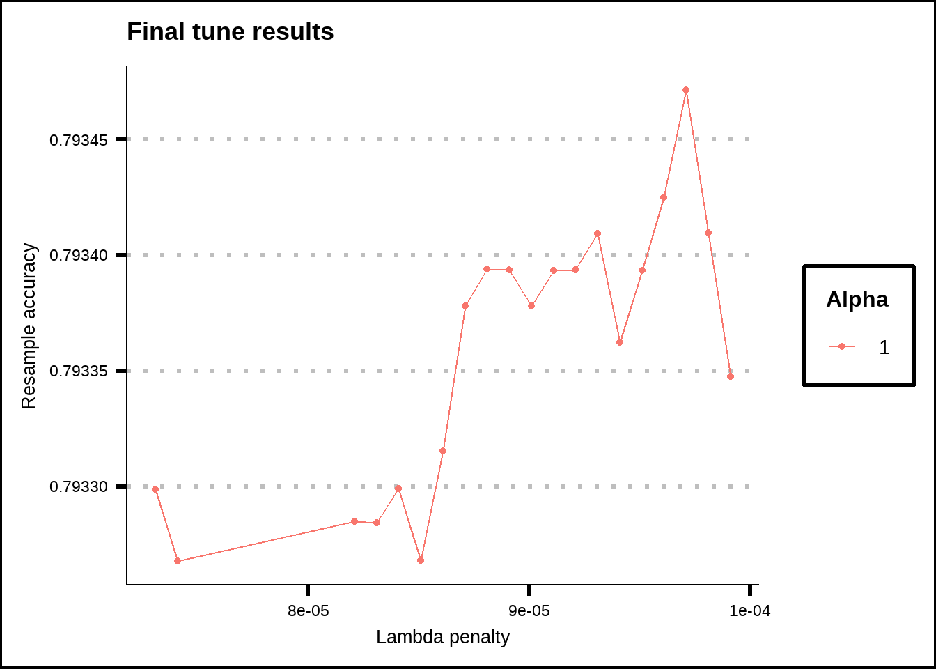
Figure 8.2: Tuning results for the GLMNET model.
8.4 Generalized additive models - GAM
gam_final_mod <- gen_additive_mod(select_features = FALSE) %>%
  set_engine("mgcv") %>%
  set_mode("classification")

f <- reformulate(setdiff(colnames(final_train), "Transported"), response = "Transported")

set.seed(8584)
gam_final_fit <- fit(object = gam_final_mod, formula = f, data = final_train)

gam_final_pred <- predict(gam_final_fit, final_test, type = "class")
gam_final_acc <- accuracy_vec(final_test$Transported, gam_final_pred$.pred_class)
8.5 SVM
The parsnip package offers three different SVM engines.
SVM_linear defines a SVM model that uses a linear class boundary. For classification, the model tries to maximize the width of the margin between classes using a linear class boundary. There is a single tuning parameter (named cost in parsnip) that determines how strict misclassification should be treated. The stricter the cost, the greater risk of overfitting.
svm_linear_final_mod <- svm_linear(cost = tune()) %>%
  set_mode("classification") %>%
  set_engine("kernlab")

svm_linear_final_wf <- glm_final_wf %>%
  update_model(svm_linear_final_mod)

my_acc <- metric_set(accuracy)
svm_linear_ctrl <- control_grid(save_pred = TRUE, save_workflow = TRUE)
svm_linear_grid <- expand.grid(cost = seq(0, 2, 0.2))

# my_cluster <- snow::makeCluster(detectCores() - 1, type = 'SOCK')
# registerDoSNOW(my_cluster)
#
# system.time({
#   set.seed(8584)
#   svm_linear_final_tune <- svm_linear_final_wf %>%
#     tune_grid(object = ., resamples = final_folds, metrics = my_acc, control = svm_linear_ctrl, grid = svm_linear_grid)
# })
#
# save(svm_linear_final_tune, file = "Extra/Final SVM linear tune.RData")
#
# snow::stopCluster(my_cluster)
# unregister()

load("Extra/Final SVM linear tune.RData")

show_best(svm_linear_final_tune, metric = "accuracy", n = 20) %>%
  ggplot(aes(x = cost, y = mean)) +
  geom_line() +
  geom_point() +
  scale_x_continuous(breaks = seq(0, 2, 0.2)) +
  labs(title = "Final tune results", x = "Cost penalty", y = "Resample accuracy")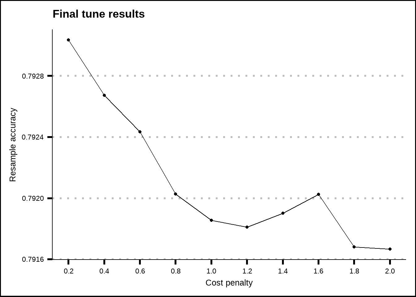
Figure 8.3: Tuning results for the SVM linear model.
set.seed(8584)
svm_linear_final_fit <- fit_best(svm_linear_final_tune)
#>  Setting default kernel parameters

svm_linear_final_pred <- predict(svm_linear_final_fit, final_test, type = "class")
svm_linear_final_acc <- accuracy_vec(final_test$Transported, svm_linear_final_pred$.pred_class)
SVM_poly model tries to maximize the width of the margin between classes using a polynomial class boundary. There are three tuning parameters in parsnip: cost, degree and scale. The cost-parameter is the same as for the linear model while the degree-parameter determines the degree of the polynomial. Lower degrees might find polynomial functions that underfit while higher might overfit. The scale factor is used to scale the data and isn’t necessary if the predictors are already scaled.
svm_poly_final_mod <- svm_poly(cost = tune(), degree = tune(), scale_factor = tune()) %>%
  set_mode("classification") %>%
  set_engine("kernlab")

svm_poly_final_wf <- glm_final_wf %>%
  update_model(svm_poly_final_mod)

my_acc <- metric_set(accuracy)
svm_poly_ctrl <- control_grid(save_pred = TRUE, save_workflow = TRUE)
svm_poly_grid <- expand.grid(cost = c(0.2, 0.6, 1), degree = c(1, 2, 3, 4), scale_factor = 1)

# my_cluster <- snow::makeCluster(detectCores() - 1, type = 'SOCK')
# registerDoSNOW(my_cluster)
#
# system.time({
#   set.seed(8584)
#   svm_poly_final_tune <- svm_poly_final_wf %>%
#     tune_grid(object = ., resamples = final_folds, metrics = my_acc, control = svm_poly_ctrl, grid = svm_poly_grid)
# })
#
# save(svm_poly_final_tune, file = "Extra/Final SVM polynomial tune.RData")
#
# snow::stopCluster(my_cluster)
# unregister()

load("Extra/Final SVM polynomial tune.RData")

show_best(svm_poly_final_tune, metric = "accuracy", n = 20) %>%
  ggplot(aes(x = as.factor(cost), y = mean, colour = as.factor(degree))) +
  geom_point() +
  scale_y_continuous(breaks = seq(0.7, 0.8, 0.01)) +
  labs(title = "Final tune results", x = "Cost penalty", y = "Resample accuracy", colour = "Polynomial\ndegree")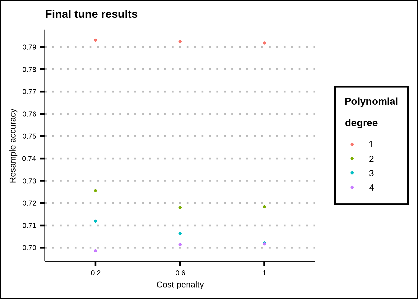
Figure 8.4: Tuning results for the SVM poly model.
set.seed(8584)
svm_poly_final_fit <- fit_best(svm_poly_final_tune)

svm_poly_final_pred <- predict(svm_poly_final_fit, final_test, type = "class")
svm_poly_final_acc <- accuracy_vec(final_test$Transported, svm_poly_final_pred$.pred_class)
SVM_rbf model stands for Radial Basis Function and tries to maximize the width of the margin between classes using a nonlinear class boundary. It is useful to predictors that overlap since it maps the data into an infinite dimension space. It has two tuning parameters: cost and \(\sigma\). The cost-parameter is the same as for the other two SVM-models while the \(\sigma\)-parameter can be seen as a weighting parameter to adjust the influence of nearby data.
svm_rbf_final_mod <- svm_rbf(cost = tune()) %>%
  set_mode("classification") %>%
  set_engine("kernlab")

svm_rbf_final_wf <- glm_final_wf %>%
  update_model(svm_rbf_final_mod)

my_acc <- metric_set(accuracy)
svm_rbf_ctrl <- control_grid(save_pred = TRUE, save_workflow = TRUE)
svm_rbf_grid <- expand.grid(cost = c(0.2, 0.6, 1, 1.2, 1.8, 3, 5))

# my_cluster <- snow::makeCluster(detectCores() - 1, type = 'SOCK')
# registerDoSNOW(my_cluster)
#
# system.time({
#   set.seed(8584)
#   svm_rbf_final_tune <- svm_rbf_final_wf %>%
#     tune_grid(object = ., resamples = final_folds, metrics = my_acc, control = svm_rbf_ctrl, grid = svm_rbf_grid)
# })
#
# save(svm_rbf_final_tune, file = "Extra/Final SVM rbf tune.RData")
#
# snow::stopCluster(my_cluster)
# unregister()

load("Extra/Final SVM rbf tune.RData")

show_best(svm_rbf_final_tune, metric = "accuracy", n = 20) %>%
  ggplot(aes(x = cost, y = mean)) +
  geom_line() +
  geom_point() +
  labs(title = "Final tune results", x = "Cost penalty", y = "Resample accuracy")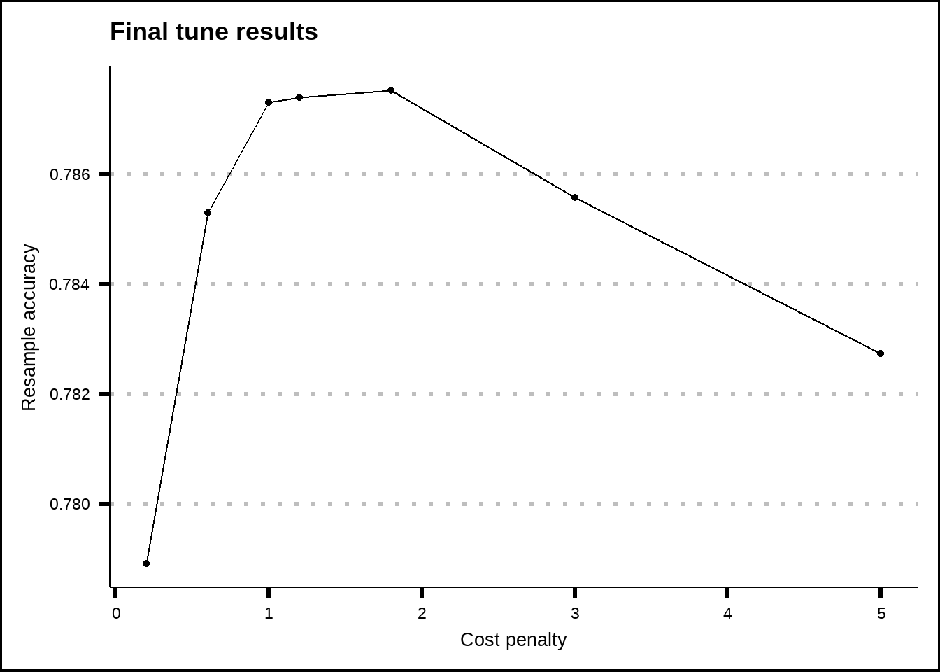
Figure 8.5: Tuning results for the SVM rbf model.
8.6 Naive Bayes
The Naive Bayes model has two tuning parameters in the parsnip package: smoothness and Laplace. The smoothness parameter controls the models class boundaries where lower values mean that the probabilities are more closely based on what we see in the training data while a higher value means that the probabilities are more smoothed (imagine points on a graph: low smoothness would draw a complex line through each point while high smoothness might draw a simple linear line - the best fit is probably somewhere in between). The Laplace-parameter can be used to add a value to the probability calculations to avoid zero probabilities in cases when variables have very low frequency values or when the test data has values not present in the training data.
nb_final_mod <- naive_Bayes(smoothness = tune(), Laplace = tune()) %>%
  set_engine("klaR") %>%
  set_mode("classification")

nb_final_wf <- glm_final_wf %>%
  update_model(nb_final_mod)

my_acc <- metric_set(accuracy)
nb_ctrl <- control_grid(save_pred = TRUE, save_workflow = TRUE)
nb_grid <- expand.grid(smoothness = seq(0, 5, 0.5), Laplace = 1)

# my_cluster <- snow::makeCluster(detectCores() - 1, type = 'SOCK')
# registerDoSNOW(my_cluster)
#
# system.time({
#   set.seed(8584)
#   nb_final_tune <- nb_final_wf %>%
#     tune_grid(object = ., resamples = final_folds, metrics = my_acc, control = nb_ctrl, grid = nb_grid)
# })
#
# save(nb_final_tune, file = "Extra/Final Naive Bayes tune.RData")
#
# snow::stopCluster(my_cluster)
# unregister()

load("Extra/Final Naive Bayes tune.RData")

show_best(nb_final_tune, metric = "accuracy", n = 20) %>%
  ggplot(aes(x = smoothness, y = mean)) +
  geom_line() +
  geom_point() +
  labs(title = "Final tune results", x = "Cost penalty", y = "Resample accuracy")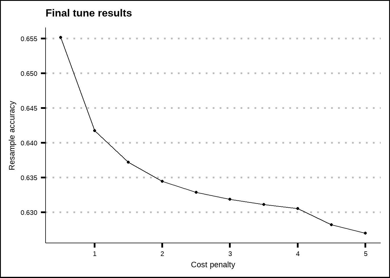
Figure 8.6: Tuning results for the Naive Bayes model.
8.7 KNN
We’ve already used the K-Nearest Neighbours function to impute data in 3, which uses a distance measure to determine how close a new observations is to its nearest neighbours. The model has two tuning parameters in parsnip: neighbors and weight_func. The neighbors-parameter is used to decide how many neighbours should be used for similarity comparison while the weigh_func-parameter is used to set the kernel that is used for the distance measure between the neighbours. There are a variety of kernels to choose from:
Rectangular: This is also known as the uniform kernel. It gives equal weight to all neighbors within the window, effectively creating a binary situation where points are either in the neighborhood (and given equal weight) or not. Triangular: This kernel assigns weights linearly decreasing from the center. It gives the maximum weight to the nearest neighbor and the minimum weight to the farthest neighbor within the window. Epanechnikov: This kernel is parabolic with a maximum at the center, decreasing to zero at the window’s edge. It is often used because it minimizes the mean integrated square error. Biweight: This is a smooth, bell-shaped kernel that gives more weight to the nearer neighbors. Triweight: This is similar to the biweight but gives even more weight to the nearer neighbors. Cos: This kernel uses the cosine of the distance to weight the neighbors. Inv: This kernel gives weights as the inverse of the distance. Gaussian: This kernel uses the Gaussian function to assign weights. It has a bell shape and does not compactly support, meaning it gives some weight to all points in the dataset, but the weight decreases rapidly as the distance increases. Rank: This kernel uses the ranks of the distances rather than the distances themselves.
For our purposes, we probably want to use the rectangular kernel to keep it simple. I’m not sure if any weighting makes sense for our type of variables and response.
knn_final_mod <- nearest_neighbor(neighbors = tune(), weight_func = "rectangular") %>%
  set_engine("kknn") %>%
  set_mode("classification")

knn_final_wf <- glm_final_wf %>%
  update_model(knn_final_mod)

my_acc <- metric_set(accuracy)
knn_ctrl <- control_grid(save_pred = TRUE, save_workflow = TRUE)
knn_grid <- expand.grid(neighbors = seq(3, 20, 1))

# my_cluster <- snow::makeCluster(detectCores() - 1, type = 'SOCK')
# registerDoSNOW(my_cluster)
#
# system.time({
#   set.seed(8584)
#   knn_final_tune <- knn_final_wf %>%
#     tune_grid(object = ., resamples = final_folds, metrics = my_acc, control = knn_ctrl, grid = knn_grid)
# })
#
# save(knn_final_tune, file = "Extra/Final KNN tune.RData")
#
# snow::stopCluster(my_cluster)
# unregister()

load("Extra/Final KNN tune.RData")

show_best(knn_final_tune, metric = "accuracy", n = 20) %>%
  ggplot(aes(x = neighbors, y = mean)) +
  geom_line() +
  geom_point() +
  labs(title = "Final tune results", x = "Cost penalty", y = "Resample accuracy")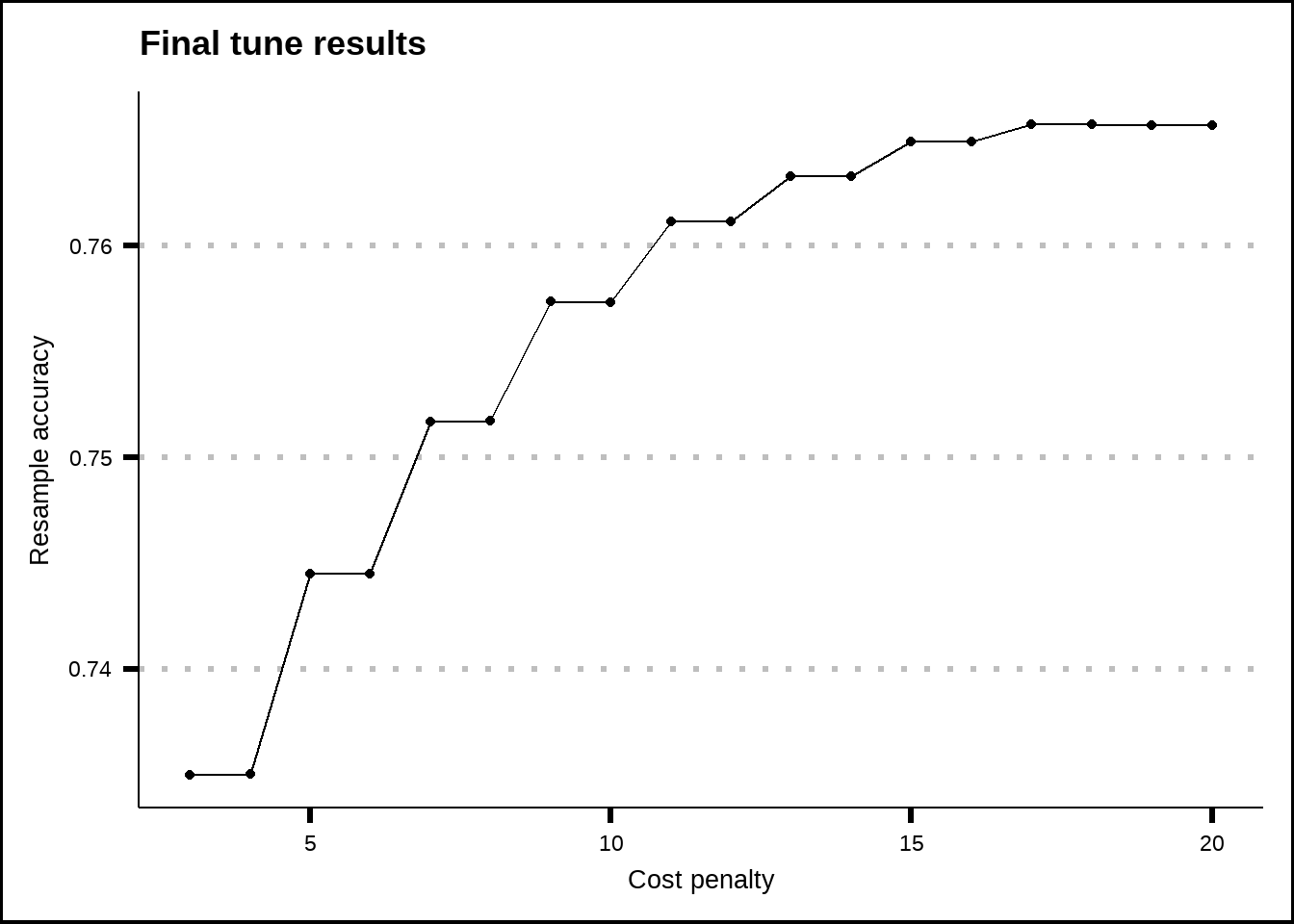
Figure 8.7: Tuning results for the KNN model.
8.8 C5
The C5.0 model for decision trees for has only a single tuning parameter in parsnip: min_n. This parameter sets the minimal node size which is a lower boundary for how many values a node must have if it is to be split further.
c5.0_final_mod <- decision_tree(min_n = tune()) %>%
  set_mode("classification") %>%
  set_engine("C5.0")

c5.0_final_wf <- glm_final_wf %>%
  update_model(c5.0_final_mod)

my_acc <- metric_set(accuracy)
c5.0_ctrl <- control_grid(save_pred = TRUE, save_workflow = TRUE)
c5.0_grid <- expand.grid(min_n = c(2, 3, 4, 5, 8, 12, 24, 48, 72, 96, 120, 144))

# my_cluster <- snow::makeCluster(detectCores() - 1, type = 'SOCK')
# registerDoSNOW(my_cluster)
#
# system.time({
#   set.seed(8584)
#   c5.0_final_tune <- c5.0_final_wf %>%
#     tune_grid(object = ., resamples = final_folds, metrics = my_acc, control = c5.0_ctrl, grid = c5.0_grid)
# })
#
# save(c5.0_final_tune, file = "Extra/Final C5_0 tune.RData")
#
# snow::stopCluster(my_cluster)
# unregister()

load("Extra/Final C5_0 tune.RData")

show_best(c5.0_final_tune, metric = "accuracy", n = 20) %>%
  ggplot(aes(x = min_n, y = mean)) +
  geom_line() +
  geom_point() +
  labs(title = "Final tune results", x = "Minimum values in leaf node", y = "Resample accuracy")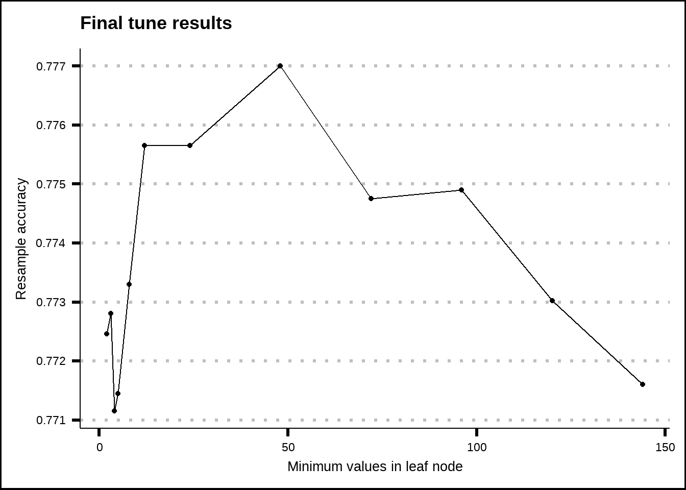
Figure 8.8: Tuning results for the C5.0 model.
8.9 RandomForest
This model has three tuning parameters: mtry, trees and min_n. The mtry-parameter sets the number of randomly selected predictors used to initiate each tree in the forest while the tree-parameter sets the maximum number of trees that are to be used. The min_n is the same as for the C5.0 model and decides the lowest number of values that must be present in a node so that it is allowed to be split. We will leave the mtry-parameter to its default value.
my_min_n <- select_best(c5.0_final_tune)$min_n

rf_final_mod <- rand_forest(trees = tune(), min_n = !!my_min_n) %>%
  set_engine("randomForest") %>%
    set_mode("classification")

rf_final_wf <- glm_final_wf %>%
  update_model(rf_final_mod)

my_acc <- metric_set(accuracy)
rf_ctrl <- control_grid(save_pred = TRUE, save_workflow = TRUE, parallel_over = "resamples")
rf_grid <- expand.grid(trees = seq(300, 800, 100))

# my_cluster <- snow::makeCluster(detectCores() - 1, type = 'SOCK')
# registerDoSNOW(my_cluster)
#
# system.time({
#   set.seed(8584)
#   rf_final_tune <- rf_final_wf %>%
#     tune_grid(., resamples = final_folds, metrics = my_acc, control = rf_ctrl, grid = rf_grid)
# })
#
# save(rf_final_tune, file = "Extra/Final randomForest tune.RData")
#
# snow::stopCluster(my_cluster)
# unregister()

load("Extra/Final randomForest tune.RData")

show_best(rf_final_tune, metric = "accuracy", n = 20) %>%
  ggplot(aes(x = trees, y = mean)) +
  geom_line() +
  geom_point() +
  scale_x_log10() +
  labs(title = "Tune results for RandomForest", x = "Number of trees", y = "Resample accuracy")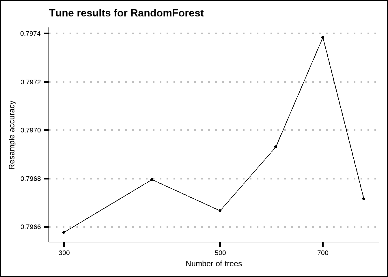
Figure 8.9: Tuning results for the RandomForest model.
8.10 XGBoost
XGBoost is a very complicated tree-based model that uses boosting where each iteration, the results of the previous iteration are used as inputs to tweak the next ensamble of trees. It has 8 tuning parameters in the parsnip package: tree_depth, trees, learn_rate, mtry, min_n, loss_reduction, sample_size and stop_iter. We can use the best values from previous tree-models for some of these and leave others to their defaults.
The ones we will tune is the tree depth, the learn-rate and the loss reduction. The tree depth sets the maxim number of splits within each tree. The learn-rate determines how large steps between boosting iterations the model takes. The larger the steps, the better the performance but the model may miss an important solution. The loss reduction determines the minimum loss that is required to further split a node of a tree. High values lead to less overfitting but also a higher risk of underfitting while low values increase the risk of overfitting.
my_min_n <- select_best(c5.0_final_tune)$min_n
my_trees <- select_best(rf_final_tune)$trees

xgb_final_mod <- boost_tree(tree_depth = tune(), learn_rate = tune(), loss_reduction = tune(),
                            min_n = !!my_min_n, trees = !!my_trees) %>%
  set_engine("xgboost") %>%
  set_mode("classification")

xgb_final_wf <- glm_final_wf %>%
  update_model(xgb_final_mod)

my_acc <- metric_set(accuracy)
xgb_ctrl <- control_grid(save_pred = TRUE, save_workflow = TRUE)
xgb_grid <- expand.grid(tree_depth = 3, learn_rate = seq(0, 0.2, 0.02), loss_reduction = seq(0, 1, 0.5))

# my_cluster <- snow::makeCluster(detectCores() - 1, type = 'SOCK')
# registerDoSNOW(my_cluster)
#
# system.time({
#   set.seed(8584)
#   xgb_final_tune <- xgb_final_wf %>%
#     tune_grid(., resamples = final_folds, metrics = my_acc, control = xgb_ctrl, grid = xgb_grid)
# })
#
# save(xgb_final_tune, file = "Extra/Final XGBoost tune.RData")
#
# snow::stopCluster(my_cluster)
# unregister()

load("Extra/Final XGBoost tune.RData")

show_best(xgb_final_tune, metric = "accuracy", n = 110) %>%
  ggplot(aes(x = learn_rate, y = mean, colour = as.factor(loss_reduction))) +
  geom_point() +
  geom_line() +
  labs(title = "Tune results for XGBoost", x = "Learn rate", y = "Resample accuracy", colour = "Loss\nreduction")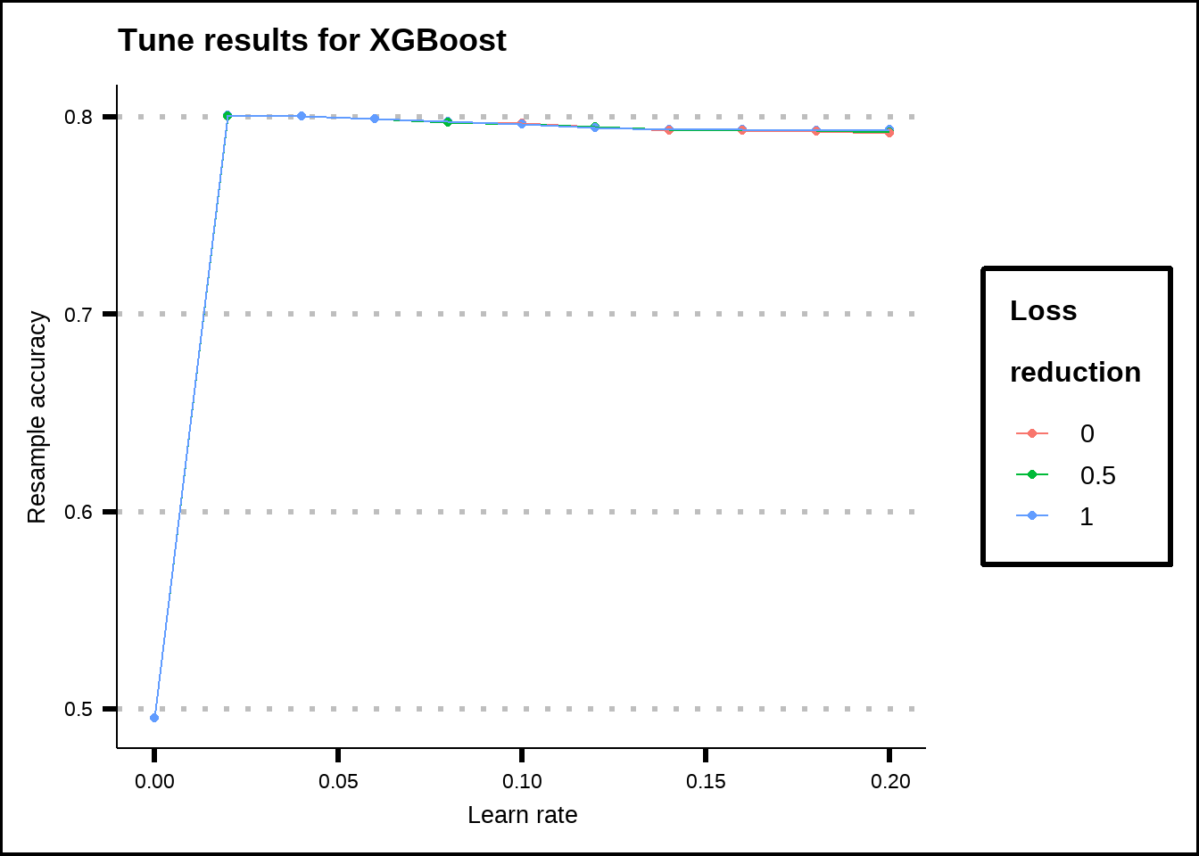
Figure 8.10: Tuning results for the XGBoost model.