7 Feature selection and elimination

Now that we have created several new features and discovered promising interaction effects, we must explore which of these have the potential to improve our models and which don’t. Kuhn and Johnson recommend several methods for feature selection and elimination that we’ll explore.

Please note that the chunks below can take many (48-96) hours to run, depending on your setup. To reduce computation time, lower the size-variables to a smaller grid search.

7.1 Recursive feature elimination

Recursive feature elimination is a process that begins with a model that includes all the features and through a systematized resampling process removes sets of variables to see whether it improves performance. The goal of the process is to converge on a set of predictor variables that produce the best results.

We’ll use all of our original variables as well as the interaction effects we’ve identified in the previous chapter.

rfe_df <- train6 %>%
  select(-c(Cabin, Name, LastName, PassengerCount, HomePlanetsPerGroup))

set.seed(8584)
rfe_split <- initial_split(rfe_df, prop = 0.8)
rfe_train <- training(rfe_split)

rfe_vars <- data.frame(Variables = names(rfe_df)) %>%
  mutate(Roles = case_when(Variables == "PassengerId" ~ "id",
                           Variables == "Transported" ~ "outcome",
                           .default = "predictor"))

int_formula <- pen_int_vars %>%
  select(ForFormula, RevFormula) %>%
  unlist() %>%
  unname() %>%
  str_flatten(., collapse = "+") %>%
  str_c("~", .) %>%
  as.formula(.)

rfe_rec <- recipe(x = rfe_train, vars = rfe_vars$Variables, roles = rfe_vars$Roles) %>%
  step_normalize(Age, RoomService, FoodCourt, ShoppingMall, Spa, VRDeck, PassengerGroup, CabinNumber, TotalSpent,
                 TotalSpentPerGroup, LastNameAsNumber) %>%
  step_dummy(all_nominal_predictors()) %>%
  step_interact(int_formula) %>%
  step_zv(all_predictors())

many_stats <- function(data, lev = levels(data$obs), model = NULL) {
    c(twoClassSummary(data = data, lev = levels(data$obs), model),
      prSummary(data = data, lev = levels(data$obs), model),
      mnLogLoss(data = data, lev = levels(data$obs), model),
      defaultSummary(data = data, lev = levels(data$obs), model))
}
rfe_funcs <- caret::caretFuncs
rfe_funcs$summary <- many_stats
rfe_funcs$fit <- function (x, y, first, last, ...) 
  train(x, y, trControl = trainControl(classProbs = TRUE), ...)
rfe_sizes <- seq(10, 350, 10)
rfe_ctrl <- rfeControl(method = "repeatedcv", repeats = 5, functions = rfe_funcs, returnResamp = "all", verbose = FALSE)

# my_cluster <- snow::makeCluster(detectCores() - 1, type = 'SOCK')
# registerDoSNOW(my_cluster)
# 
# snow::clusterEvalQ(my_cluster, library(recipes))
# snow::clusterExport(my_cluster, "int_formula")
# 
# system.time({
#   set.seed(8584)
#   rfe_acc <- rfe(rfe_rec, data = rfe_train, method = "glm", family = "binomial", metric = "Accuracy", sizes = rfe_sizes,
#                  rfeControl = rfe_ctrl)
# })
# 
# save(rfe_acc, file = "Extra/Recursive feature elimination with interactions.RData")
# 
# stopCluster(my_cluster)
# unregister()

load("Extra/Recursive feature elimination with interactions.RData")

rfe_avg_res <- rfe_acc$results %>%
  select(Variables, Accuracy)

rfe_avg_res %>%
  ggplot(data = ., aes(x = Variables, y = Accuracy)) +
  geom_point() +
  geom_line() +
  geom_vline(xintercept = 110, linetype = "dashed", colour = "blue", size = 1)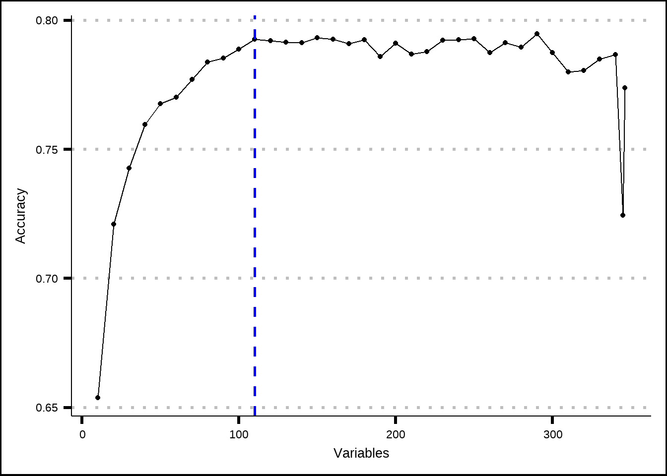

Figure 7.1: Estimated performance with recursive feature elimination based on the number of variables that are included.

The results for the RFE-process indicate is that the accuracy doesn’t improve beyond 110 variables. Let’s save those.

rfe_best <- rfe_acc[["variables"]] %>%
  filter(Variables == 110) %>%
  select(var, Resample) %>%
  nest(.by = Resample) %>%
  left_join(., rfe_acc[["resample"]] %>% 
              filter(Variables == 110) %>% 
              select(Accuracy, Resample),
            by = "Resample")

rfe_best_vars <- rfe_best %>%
  filter(Accuracy == max(Accuracy)) %>%
  pull(data) %>%
  unlist(.)

names(rfe_best_vars) <- rfe_best_vars

7.2 Simulated annealing

Kuhn and Johnson describe the process of simulated annealing in detail in their book but the main purpose is to iterate over random subsets of predictor variables and calculate performance until an optimal set is found. The process starts from a given set of variables and then adds or removes subsets and evaluates if these add to the performance. If they do, the new subset its kept and tested against others. The process uses randomness to avoid converging on a subset of variables that has high performance in a particular resample (local optima).

We’ll use the same setup as we did for the recursive feature elimination above. We initiate the process with a random subset of 30% of the variables.

sa_df <- train6 %>%
  select(-c(Cabin, Name, LastName, PassengerCount, HomePlanetsPerGroup))

set.seed(8584)
sa_split <- initial_split(sa_df, prop = 0.8)
sa_train <- training(sa_split)

sa_vars <- data.frame(Variables = names(sa_df)) %>%
  mutate(Roles = case_when(Variables == "PassengerId" ~ "id",
                           Variables == "Transported" ~ "outcome",
                           .default = "predictor"))

int_formula <- pen_int_vars %>%
  select(ForFormula, RevFormula) %>%
  unlist() %>%
  unname() %>%
  str_flatten(., collapse = "+") %>%
  str_c("~", .) %>%
  as.formula(.)

sa_rec <- recipe(x = sa_train, vars = sa_vars$Variables, roles = sa_vars$Roles) %>%
  step_normalize(Age, RoomService, FoodCourt, ShoppingMall, Spa, VRDeck, PassengerGroup, CabinNumber, TotalSpent,
                 TotalSpentPerGroup, LastNameAsNumber) %>%
  step_dummy(all_nominal_predictors()) %>%
  step_interact(int_formula) %>%
  step_zv(all_predictors())

sa_bake <- sa_rec %>% prep() %>% bake(new_data = NULL)

sa_funcs <- caretSA
sa_funcs$fitness_extern <- many_stats
sa_funcs$initial <- function(vars, prob = 0.30, ...) { # Change the prob to begin from a lower or higher subset
  sort(sample.int(vars, size = floor(vars * prob) + 1))
}

# Inner control
sa_ctrl_inner <- trainControl(method = "boot", p = 0.90, number = 1, summaryFunction = many_stats, classProbs = TRUE, 
                        allowParallel = FALSE)

# Outer control for SA
sa_ctrl_outer <- safsControl(method = "cv", metric = c(internal = "Accuracy", external = "Accuracy"), 
                       maximize = c(internal = TRUE, external = TRUE), functions = sa_funcs, improve = 20, returnResamp = "all",
                       verbose = FALSE, allowParallel = TRUE)

# my_cluster <- snow::makeCluster(detectCores() - 1, type = 'SOCK')
# registerDoSNOW(my_cluster)
# snow::clusterExport(cl = my_cluster, "int_formula")
# 
# system.time({
#   set.seed(8485)
#   sa_30pct_init <- safs(sa_rec, data = sa_train, iters = 500, safsControl = sa_ctrl_outer, method = "glm",
#                             trControl = sa_ctrl_inner, metric = "Accuracy")
# })
# 
# save(sa_30pct_init, file = "Extra/Simulated annealing.RData")
# 
# snow::stopCluster(my_cluster)
# unregister()

load("Extra/Simulated annealing.RData")

sa_acc_int <- sa_30pct_init$internal
sa_acc_int2 <- sa_acc_int %>%
  group_by(Iter) %>%
  summarise(Accuracy = sum(Accuracy) / length(unique(sa_acc_int$Resample))) %>%
  ungroup() %>%
  mutate(Resample = "Averaged") %>%
  bind_rows(sa_acc_int, .) %>%
  mutate(colour_grp = if_else(Resample == "Averaged", "yes", "no"))

sa_avg_int <- sa_acc_int2 %>% filter(Resample == "Averaged") %>% select(Iter, Accuracy)
  
ggplot(sa_acc_int2, aes(x = Iter, y = Accuracy, colour = colour_grp)) +
  geom_point() +
  facet_wrap(~Resample) +
  theme(legend.position = "none")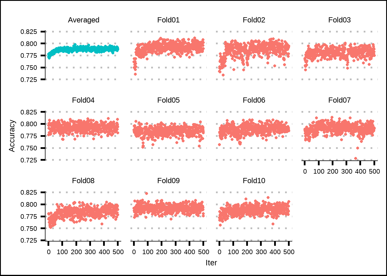

Figure 7.2: Estimated performance of internal resamples from simulated annealing.

The results from the internal simulated annealing process suggest that our initial random set of 30% of the variables has relatively high accuracy but that some improvement is made through the iterations, based on how the average accuracy increasesfor the first 100 iterations.

sa_acc_ext <- sa_30pct_init$external
sa_acc_ext2 <- sa_acc_ext %>%
  group_by(Iter) %>%
  summarise(Accuracy = sum(Accuracy) / length(unique(sa_acc_ext$Resample))) %>%
  ungroup() %>%
  mutate(Resample = "Averaged") %>%
  bind_rows(sa_acc_ext, .) %>%
  mutate(colour_grp = if_else(Resample == "Averaged", "yes", "no"))

sa_avg_ext <- sa_acc_ext2 %>% filter(Resample == "Averaged") %>% select(Iter, Accuracy)

ext_int_corr <- round(cor(sa_avg_int$Accuracy, sa_avg_ext$Accuracy), 2)

ggplot(mapping = aes(x = Iter, y = Accuracy)) +
  geom_point(data = sa_avg_int, aes(colour = "Internal")) +
  geom_point(data = sa_avg_ext, aes(colour = "External")) +
  geom_label(data = sa_avg_ext, x = 5, y = 0.795, label = str_c("Corr: ", ext_int_corr)) +
  labs(colour = "Estimate") +
  scale_colour_manual(values = c("Internal" = "red", "External" = "green"))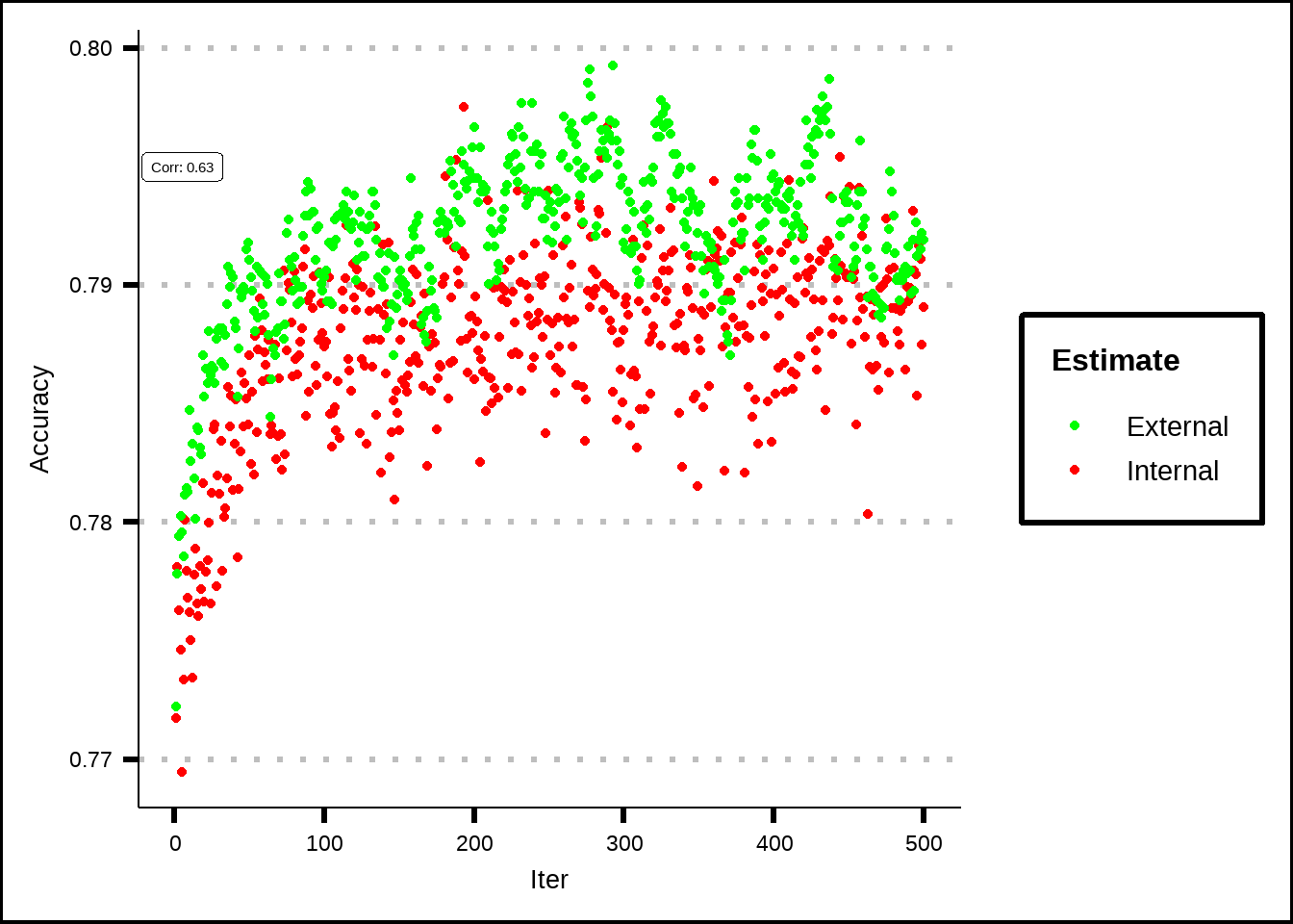

Figure 7.3: Estimated performance of external resamples from simulated annealing.

The external resampling is used to check performance for different iterations and since it correlates relatively well with the internal resamples, we can conclude that the internal resamples haven’t overfitted to the data.

sa_final <- sa_30pct_init$sa
sa_final2 <- data.frame(Iter = sa_final[["internal"]]$Iter, Accuracy = sa_final[["internal"]]$Accuracy,
                                Subset_Size = unlist(lapply(sa_final[["subsets"]], length))) %>%
  pivot_longer(-Iter)

ggplot(sa_final2, aes(x = Iter, y = value)) +
  geom_point() +
  geom_vline(xintercept = 488, linetype = "dashed", colour = "blue", size = 1, alpha = 0.6) +
  facet_wrap(~name, nrow = 2, ncol = 1, scales = "free_y")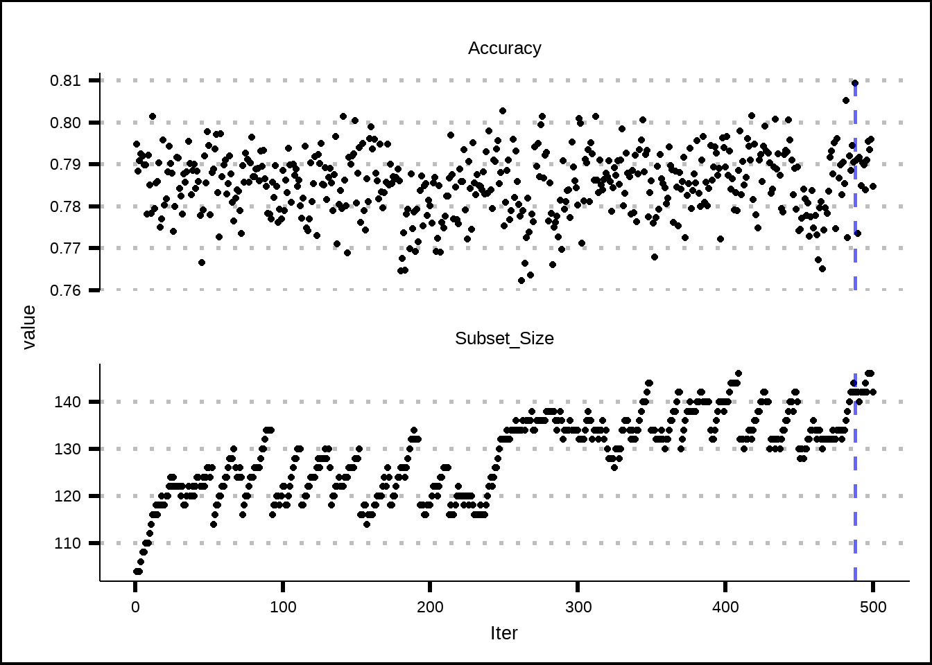

Figure 7.4: Estimated performance of best resample from simulated annealing.

The final results from the simulated annealing process indicate that a subset of 142 variables produces the best accuracy, which is close to 0.81. It is possible that more iterations would’ve revealed further improvements but since this subset is close to the one produced from the RFE-model (110), we’ll assume that the number of iterations were enough.

Let us save the best variables from the process for possible later use.

sa_best_vars <- sa_30pct_init[["optVariables"]]

7.3 Genetic algorithm

The final process for feature selection that we’ll use is a genetic algorithm. Similar to simulated annealing, it starts with a subset of variables as the first generation and then iterates over different generation (external resampling) while it selects subsets of variables for ‘mating’ to see whether the new “offspring” improves performance. The process also involves steps to avoid local optima.

ga_df <- train6 %>%
  select(-c(Cabin, Name, LastName, PassengerCount, HomePlanetsPerGroup))

set.seed(8584)
ga_split <- initial_split(ga_df, prop = 0.8)
ga_train <- training(ga_split)

ga_vars <- data.frame(Variables = names(ga_df)) %>%
  mutate(Roles = case_when(Variables == "PassengerId" ~ "id",
                           Variables == "Transported" ~ "outcome",
                           .default = "predictor"))

int_formula <- pen_int_vars %>%
  select(ForFormula, RevFormula) %>%
  unlist() %>%
  unname() %>%
  str_flatten(., collapse = "+") %>%
  str_c("~", .) %>%
  as.formula(.)

ga_rec <- recipe(x = ga_train, vars = ga_vars$Variables, roles = ga_vars$Roles) %>%
  step_dummy(all_nominal_predictors()) %>%
  step_interact(int_formula) %>%
  step_zv(all_predictors()) %>%
  step_corr(all_numeric_predictors(), threshold = 0.5)

ga_funcs <- caretGA
ga_funcs$fitness_extern <- many_stats

# Inner control
ga_ctrl_inner <- trainControl(method = "boot", p = 0.90, number = 1, summaryFunction = many_stats, classProbs = TRUE,
                        allowParallel = FALSE)

# Outer control for SA
ga_ctrl_outer <- gafsControl(method = "cv", metric = c(internal = "Accuracy", external = "Accuracy"),
                       maximize = c(internal = TRUE, external = TRUE), functions = ga_funcs, returnResamp = "all",
                       verbose = FALSE, allowParallel = TRUE)

# my_cluster <- snow::makeCluster(detectCores() - 1, type = 'SOCK')
# registerDoSNOW(my_cluster)
# snow::clusterExport(cl = my_cluster, "int_formula")
# 
# system.time({
#   set.seed(8584)
#   ga_acc <- gafs(ga_rec, data = ga_train, iters = 50, gafsControl = ga_ctrl_outer, method = "glm",
#                  trControl = ga_ctrl_inner, metric = "Accuracy")
# })
# 
# save(ga_acc, file = "Extra/Genetic algorithm feature selection.RData")
# 
# snow::stopCluster(my_cluster)
# unregister()

load("Extra/Genetic algorithm feature selection.RData")

ga_acc_int <- ga_acc$internal
ga_acc_int2 <- ga_acc_int %>%
  group_by(Iter) %>%
  summarise(Accuracy = sum(Accuracy) / length(unique(ga_acc_int$Resample))) %>%
  ungroup() %>%
  mutate(Resample = "Averaged") %>%
  bind_rows(ga_acc_int, .) %>%
  mutate(colour_grp = if_else(Resample == "Averaged", "yes", "no"))

ga_avg_int <- ga_acc_int2 %>% filter(Resample == "Averaged") %>% select(Iter, Accuracy)
  
ggplot(ga_acc_int2, aes(x = Iter, y = Accuracy, colour = colour_grp)) +
  geom_point() +
  facet_wrap(~Resample) +
  theme(legend.position = "none")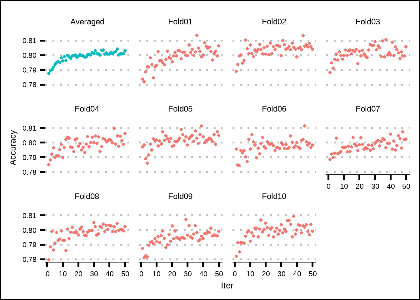

Figure 7.5: Estimated performance of internal resamples from the genetic algorithm.

The inner resamples of the genetic algorithm suggest a plateau after around twenty generations (iterations).

ga_acc_ext <- ga_acc$external
ga_acc_ext2 <- ga_acc_ext %>%
  group_by(Iter) %>%
  summarise(Accuracy = sum(Accuracy) / length(unique(ga_acc_ext$Resample))) %>%
  ungroup() %>%
  mutate(Resample = "Averaged") %>%
  bind_rows(ga_acc_ext, .) %>%
  mutate(colour_grp = if_else(Resample == "Averaged", "yes", "no"))

ga_avg_ext <- ga_acc_ext2 %>% filter(Resample == "Averaged") %>% select(Iter, Accuracy)

ga_ext_int_corr <- round(cor(ga_avg_int$Accuracy, ga_avg_ext$Accuracy), 2)

ggplot(mapping = aes(x = Iter, y = Accuracy)) +
  geom_point(data = ga_avg_int, aes(colour = "Internal")) +
  geom_point(data = ga_avg_ext, aes(colour = "External")) +
  geom_label(data = ga_avg_ext, x = 5, y = 0.803, label = str_c("Corr: ", ga_ext_int_corr)) +
  labs(colour = "Estimate") +
  scale_colour_manual(values = c("Internal" = "red", "External" = "green"))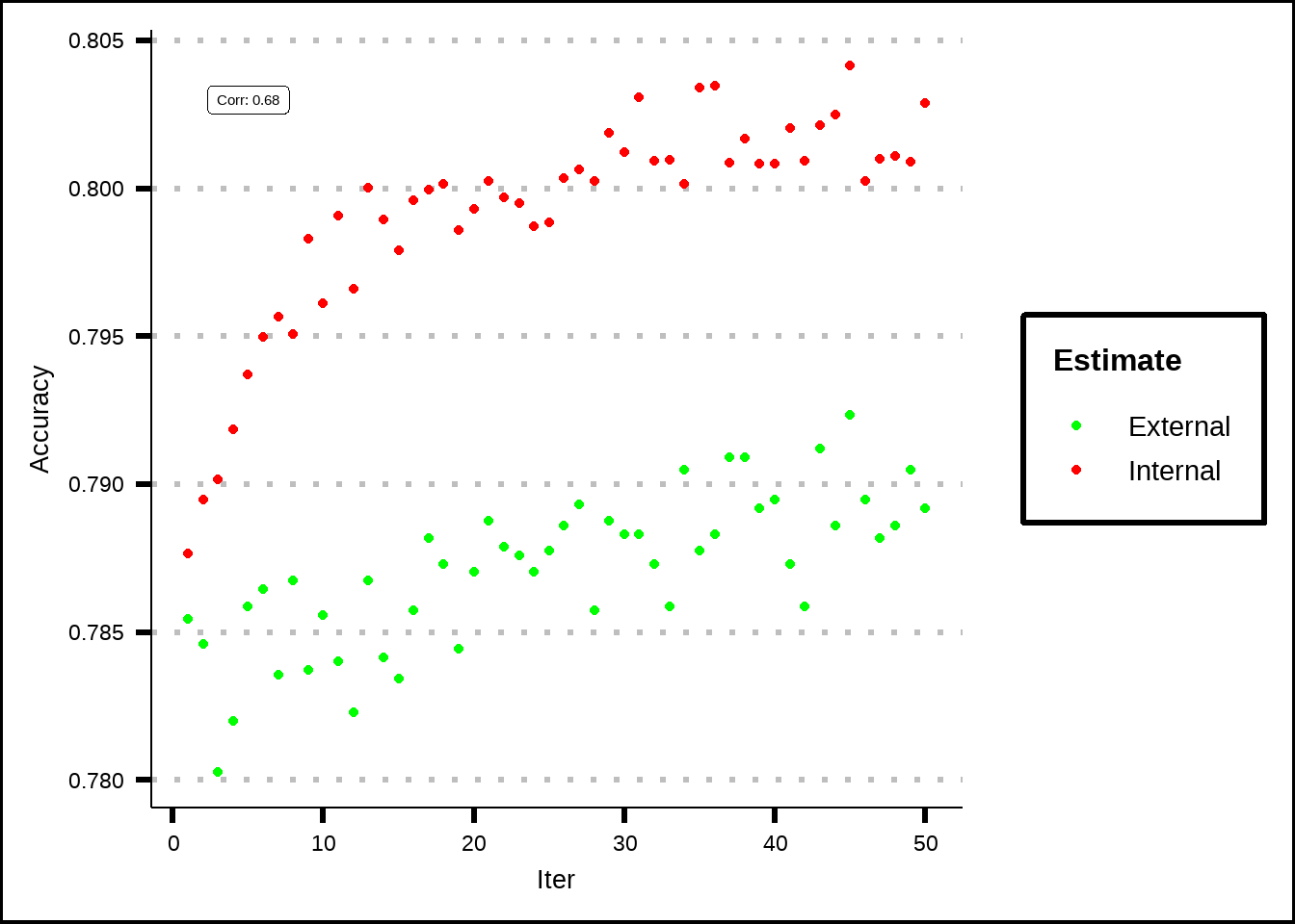

Figure 7.6: Estimated performance of external resamples from the genetic algorithm.

For the genetic algorithm, we see that the internal folds got better results which could indicate that the selections of subsets of variables (the populations) overfit to the data while the external validations (number of generations) found a more general population mix that hopefully better describes the unseen data.

Let’s save the best variables from this process for possible later use.

ga_best_vars <- ga_acc[["optVariables"]]

7.4 Check performance with random subsets

The results of our three feature selection processes suggest that the optimal set of variables (including dummy variables and their interactions) is between 110 (RFE) and 174 (SA) with the genetic algorithm coming in between these at 136.

To get a sense of how well these processes have selected subsets of variables, we can run an iteration that takes random subsets and evaluates performance. This will tell us if the processes are better than random chance. We’ll use the smallest subset (RFE) to reduce the computational demands.

rand_subset_size <- length(rfe_best_vars)

rfe_bake <- rfe_rec %>%
  prep() %>%
  bake(new_data = NULL) %>%
  select(-PassengerId)

full_vars <- rfe_bake %>% names(.)
half_full_vars <- round(length(full_vars) / 2, 0)
map_seq <- 1:half_full_vars # Number of iterations half of total number of variables to ensure sufficient combinations

rand_subset <- map(map_seq, .f = \(x) sample(full_vars, rand_subset_size))
rand_data <- map(rand_subset, .f = \(x) rfe_bake %>% dplyr::select(Transported, x))
rand_rec <- map(rand_data, .f = \(df) recipe(Transported ~ ., data = df))

subset_ctrl <- trainControl(method = "cv", classProbs = TRUE, summaryFunction = many_stats)

# my_cluster <- snow::makeCluster(detectCores() - 1, type = 'SOCK')
# registerDoSNOW(my_cluster)
# 
# system.time({
#   subset_model <- map2(.x = rand_rec, .y = rand_data,
#                        .f = \(rec, df) train(rec, data = df, method = "glm", trControl = subset_ctrl, metric = "Accuracy"))
# })
# 
# subset_perf <- map(subset_model, .f = \(m) getTrainPerf(m))
# 
# save(subset_perf, file = "Extra/Random subsets performance.RData")
# 
# snow::stopCluster(my_cluster)
# unregister()

load("Extra/Random subsets performance.RData")

rf_random_avg <- map_dbl(subset_perf, .f = \(x) x$TrainAccuracy) %>%
  enframe()

ggplot() +
  geom_point(data = rfe_avg_res, aes(x = Variables, y = Accuracy, colour = "RFE")) +
  geom_point(data = sa_avg_ext, aes(x = Iter, y = Accuracy, colour = "SA")) +
  geom_point(data = ga_avg_ext, aes(x = Iter, y = Accuracy, colour = "GA")) +
  geom_point(data = rf_random_avg, aes(x = name, y = value, colour = "Random")) +
  scale_colour_manual(values = c("RFE" = "green", "RFE Tree" = "blue", "SA" = "orange", "GA" = "red", "Random" = "darkgrey")) +
  labs(x = "Variables(RFE) or iterations", y = "Accuracy", colour = "Method") +
  lims(y = c(0.6, 0.8))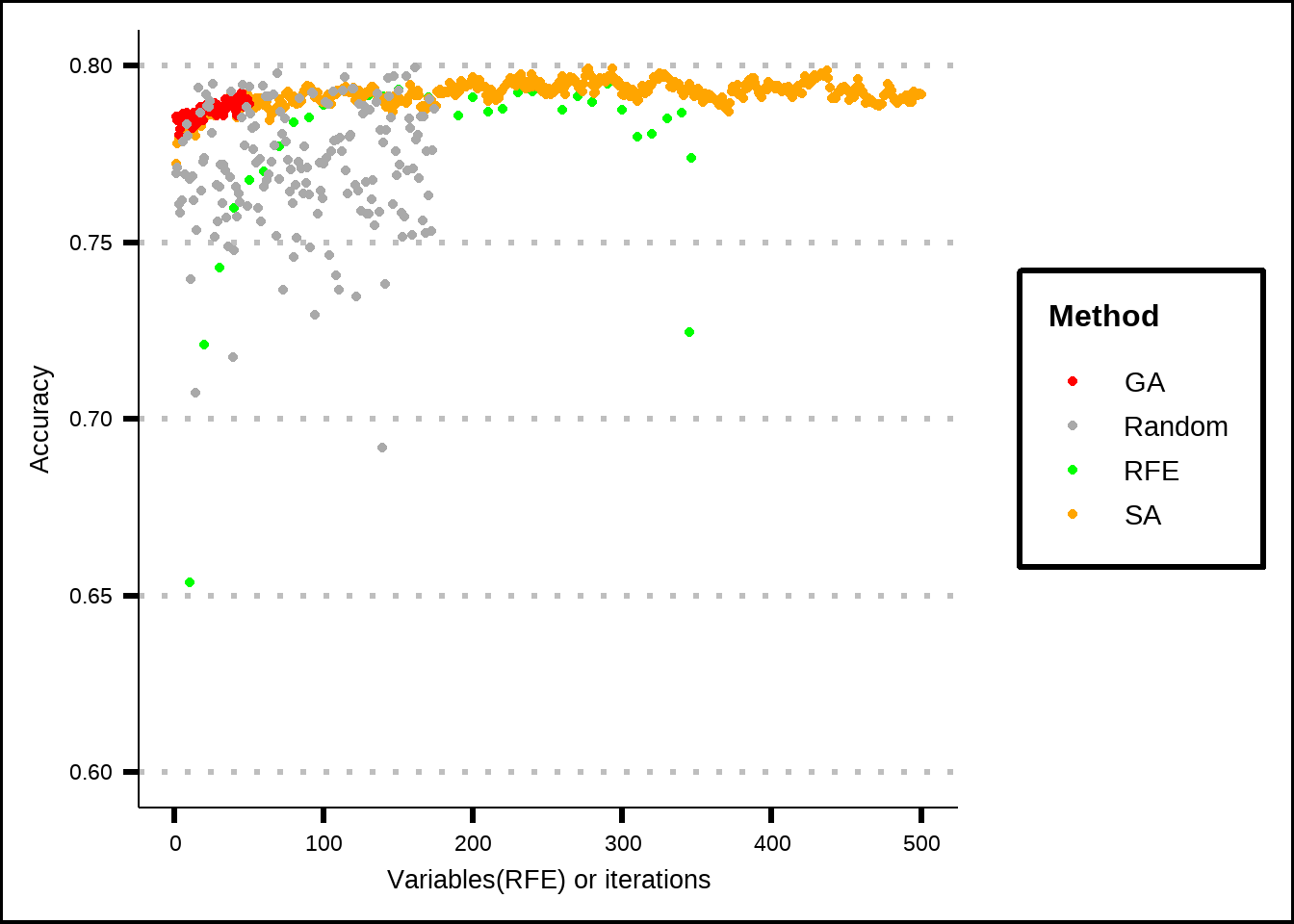

Figure 7.7: Comparison of different feature selection results against a random subset result.

It seems visually that all of our feature selection methods outperform random variable subsets most of the time but let’s quantify the differences and test for significance.

my_sample_size <- length(rf_random_avg$name)

random_avg_acc <- rf_random_avg$value
rfe_avg_acc <- sample(rfe_avg_res$Accuracy, my_sample_size, replace = TRUE)
sa_avg_acc <- sample(sa_avg_ext$Accuracy, my_sample_size, replace = TRUE)
ga_avg_acc <- sample(ga_avg_ext$Accuracy, my_sample_size, replace = TRUE)

p_wilcox_rfe <- wilcox.test(x = rfe_avg_acc, y = random_avg_acc, paired = TRUE, alternative = "greater")$p.value
p_ttest_rfe <- t.test(x = rfe_avg_acc, y = random_avg_acc, paired = TRUE, alternative = "greater")$p.value

p_wilcox_sa <- wilcox.test(x = sa_avg_acc, y = random_avg_acc, paired = TRUE, alternative = "greater")$p.value
p_ttest_sa <- t.test(x = sa_avg_acc, y = random_avg_acc, paired = TRUE, alternative = "greater")$p.value

p_wilcox_ga <- wilcox.test(x = ga_avg_acc, y = random_avg_acc, paired = TRUE, alternative = "greater")$p.value
p_ttest_ga <- t.test(x = ga_avg_acc, y = random_avg_acc,  paired = TRUE, alternative = "greater")$p.value

p_tests <- data.frame(test = rep(c("Wilcoxon paired", "t.test paired"), 3),
                      colour_grp = rep(c("RFE", "SA", "GA"), 2),
                      value = c(p_wilcox_rfe, p_wilcox_sa, p_wilcox_ga,
                                p_ttest_rfe, p_ttest_sa, p_ttest_ga))

ggplot(p_tests, aes(x = test, y = value, colour = colour_grp)) +
  geom_point(size = 5) +
  geom_hline(yintercept = 0.05, linetype = "dashed", colour = "red", show.legend = FALSE) +
  scale_colour_manual(values = c("RFE" = "green", "SA" = "orange", "GA" = "red", "size" = "none")) +
  labs(x = "Tests of difference", y = "P value", colour = "Method")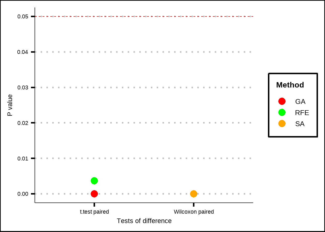

Figure 7.8: Tests if significance between different feature selection methods and random samples. The figure shows that medians (Wilcoxon) and means(t-test) for accuracy are significantly higher for results produced by the methods compared to the ones produced by random subsets.

The Wilcoxon test checks whether the median of the difference in accuracy between a processed sample and a random sample are significant and it doesn’t require the distribution of the differences between the paired samples to be normal. The t.test compares the means and does require the sample differences to be relatively normal. The null hypothesis in both cases is that the accuracies from the processed samples are smaller or equal to accuracies from random samples and so low p-values mean that the processed samples have significantly greater accuracies that random samples.

We see that all of the methods have significant improvement over the random sample and if we look back at Figure 7.7, we can see that the accuracy results seem to be comparable between the methods. Let’s therefore save the variables from the SA process since they offered the best results.

best_vars <- sa_best_vars
save(best_vars, file = "Extra/Best variables.RData")